Module 2 Sampling design for soil surveys

2.1 Introduction

Soil surveys play a critical role in environmental monitoring, evaluating soil degradation, and formulating sustainable land use strategies (Bui, 2020). They offer essential information on soil characteristics, including texture, structure, pH levels, organic matter content, nutrient availability, and other physicochemical attributes of interest. These data are essential for making informed choices about crop selection, fertilizer use, irrigation planning, and soil conservation and management strategies. Therefore, soil information and data are key components in any comprehensive soil survey that supplies necessary information for soil management decisions at local to global scales. In this sense, the Soil Mapping for Resilient Agrifood Systems (SoilFER) framework aims to provide an open-access soil information system to support the formulation of digital soil maps, fertilizer recommendations, establish crop suitability, determine soil quality indicators, assess soil health, implement soil conservation practices, and create a national soil spectral library.

State-of-the-art soil sampling protocols adopt a systematic approach that considers factors such as soil variability, sampling depth, land-use, farming activities, and sampling density (Brevik et al., 2016; Clay et al., 2001; Morton and Heinemeyer, 2000; Norris et al., 2013). This chapter provides general guidance on soil sampling design methodologies to ensure precision, reproducibility, and reliability in the collection of soil samples for digital soil mapping and monitoring. It presents a three-stage hierarchical hybrid method incorporating both probability and non-probability sampling for soil mapping and monitoring within the SoilFER framework. At the first and second hierarchical levels, the primary and secondary sampling units are selected using a covariate space coverage sampling method based on environmental covariates (model-based). At the third hierarchical level, the tertiary sampling units are selected using simple random sampling without replacement (design-based). This sampling approach standardizes soil sampling methodologies across the countries participating in the project.

2.2 Sampling methodologies for soil spatial survey

Soil monitoring and mapping are essential to understand soil variability and manage soil resources efficiently. In this context, it is important to understand the basics of choosing a sampling methodology that best fits the project’s objectives, whether focused on mapping, monitoring, or a combination of both. This section provides an overview of key sampling design concepts, presented in a manner accessible for both academic and non-academic audiences. Let’s take a look!

2.2.1 Selection of the sampling methodology

Purposive (also known as traditional or expert) and probability sampling are the most used methods for selecting sampling units in soil surveys. Both methods differ basically in their objectives. In simple terms, expert sampling involves selecting specific points along a slope or landscape feature, either at individual locations or along transects, such as a catena or toposequence. This approach aims to capture the relationships between the variation in soil properties and the different geographical features that make up the landscape. This concept has been widely used, as stated in the literature, for soil mapping (Borden, Thomas and Rivard, 2020; Gobin, Campling and Feyen, 2001; Milne, 1936). This selection method effectively captures local variations in soil properties and is useful for understanding how these properties change in relation to terrain and hydrological characteristics. However, this sampling method may not always reflect the overall variability of soil properties across the entire study area. Moreover, implementing this approach generally requires significant effort, time, and funding, particularly for large study areas.

On the other hand, probability sampling assigns a known probability of selection to each sampling unit, ensuring that each sampling unit has a chance of being included in the sample. This approach focuses on obtaining representative samples to make unbiased inferences about the entire population under study (Gruijter et al., 2006). This method requires careful planning and implementation to ensure that the sampling design is both unbiased and representative of the population. In addition, its implementation can be more complex compared to the expert sampling method. However, its main advantage is that every sampling unit has a chance of being included in the sample, resulting in a more representative sample of the variability in the study area. Additionally, it allows statistical inferences about the entire population from the sample. This last aspect, if not the most important, allows soil surveyors to monitor and better report the current and future status of soil properties. In general, traditional/expert (i.e., non-probabilistic) sampling is less flexible than probabilistic sampling since the latter allows for both types of inference methods, as we will see in the next subsection.

2.2.2 Inference Methods

Two primary statistical inference methods are used in soil survey: design- and model-based inference approaches (Gruijter et al., 2006). Design-based inference utilises the sample design to make inferences about the entire population, including probabilities of the sampling units. This approach is suitable for estimating global quantities, such as means and totals, or local quantities for large domains based on the design of the sampling scheme. Briefly, global quantities encompass the spatial cumulative distribution function of the response variable in the sampling universe, or quantities derived from it, such as quantiles, median, mean, and standard deviation. Local quantities, on the other hand, pertain to individual estimates within sub-areas of the sampling universe, also known as domains. Model-based inference uses statistical models to make inferences about unsampled locations based on the relationships observed in the sampled data. This approach is valuable for predicting soil properties at unsampled locations, especially in areas where sampling is limited. Further information about design- and model-based approaches can be found in Brus, Kempen and Heuvelink (2011 a). In simple words, the difference between them lies in where the uncertainty comes from and how conclusions are drawn.

For instance, in design-based inference, sampling locations are selected using a probability sampling design, such as simple random sampling without replacement. Every location in the study area has a known and non-zero probability of being selected. In this framework, randomness arises from the sampling process itself. The sampled data are then used to estimate characteristics of the entire study area. The validity of the results therefore depends on how well the sampling design was constructed and implemented. If the design is appropriate and correctly applied, the resulting estimates are unbiased, regardless of the spatial pattern of the soil property. Design-based inference can also be used to estimate values for sub-areas, or domains, provided that the sampling design ensures sufficient representation within those areas. In simple terms, the sample represents the whole study area if the sampling is random and properly designed. This approach is particularly useful for estimating population summaries (i.e., monitoring), such as mean soil organic carbon or total nutrient stocks.

In contrast, model-based inference begins by collecting soil samples at selected locations and then fitting a statistical model that relates soil properties to environmental covariates, such as elevation, slope, or climate variables. The fitted model is subsequently used to predict soil properties at unsampled locations. In this case, randomness arises from the assumptions of the statistical model rather than from the sampling design. The validity of the inference depends on how well the model captures the relationship between the soil property and the explanatory variables (i.e., environmental covariates). If the model is appropriate, it can be used to generate continuous prediction maps across the entire study area. In simple terms, soil properties can be predicted everywhere if the model correctly describes the underlying relationships. This approach is particularly useful for spatial prediction and for filling gaps in areas where no samples were collected.

Summary

• Monitoring: design-based inference is generally preferred.

• Mapping: model-based inference is generally preferred.

• Hybrid designs: combine both strengths.

2.2.3 Purpose of Sampling

Bounding together selection and inference methods, one can better determine which one of those combinations works best for their project goals. The choice of sampling method in soil survey and monitoring depends on the survey’s purpose (Brus, 2022 b). For monitoring soil properties over time, design-based inference and probability sampling selection are suitable. These methods allow for the unbiased estimation of changes in soil properties at specific locations over time. For mapping soil properties across a landscape, model-based inference and non-probabilistic sampling are more appropriate. These methods allow for the spatial prediction of soil properties at unsampled locations based on the relationships observed in the sampled data. Monitoring differs from estimating soil parameters of domains at a given point in time. However, similar to monitoring, design-based inference and probability sampling are the most suitable methods for estimating soil properties within a certain domain. These approaches ensure that the estimates of soil parameters (e.g., mean, variance, mode, median) are unbiased and representative of the study area.

2.2.4 Sampling Design Types

The sequence of decision-making for a soil survey or monitoring project should follow a logical order to ensure that the objectives of the project are met effectively. Begin by defining the purpose of the project. Determine whether the goal is to monitor changes in soil properties over time or to map them across the landscape. Based on the purpose, one can choose an appropriate selection method. After that, one can select the inference method that best suits the project. For instance, if the goal is monitoring, consider probability sampling. For mapping, consider either non-probability or probability methods. Once the purpose, selection and inference methods are defined, one can select the appropriate sampling design.

Before diving into the types of sampling design, it is important to consider the stratification of the sampling universe. Stratification involves dividing the sampling universe into strata or sub-areas based on certain criteria, such as soil-climate types or land-use. This approach can improve the efficiency of the sampling design by obtaining separate estimates for each stratum, leading to more precise estimates for specific regions of interest (ROI). For example, if the ROI has distinct soil types, stratifying the sample by soil type can ensure that each soil type is adequately represented in the sample. Another example is using explanatory variables (i.e., environmental covariates) from remote sensing as a means of spatial coverage and stratification.

Stratification is not a separate sampling design type; rather it is a structural feature that can be incorporated into different sampling designs to improve efficiency, representativeness, and precision. In other words, stratification modifies how a design is implemented, not the fundamental logic of the design itself. For clarity, sampling design types can be broadly grouped according to whether the primary objective is monitoring or mapping (Table 2.1). For monitoring, one can certainly choose among simple random sampling (SRS), stratified SRS, or two-stage cluster random sampling. In SRS, each sampling unit in the ROI has equal probability of being selected. This approach is straightforward and easy to implement but may not account for spatial variability in soil properties. Stratified simple random sampling divides the ROI into strata based on certain criteria, such as soil-climate types or land use. Then, SRS is conducted within each stratum. This method ensures that each stratum is adequately represented in the sample, leading to more precise estimates for specific ROI. Finally, in two-stage cluster random sampling, the sampling units are grouped into clusters, and then clusters are randomly selected for sampling. This method is useful for large study areas where it may be impractical to sample every unit individually.

An important concept that can be incorporated into these probability-based designs is balanced acceptance sampling (BAS) (Robertson et al., 2013). BAS is not a separate design category but rather a strategy that promotes spatial balance within a probability sampling framework. It can be applied within simple random, stratified, or cluster sampling to ensure that selected sampling units are well distributed across the study area or across strata. By improving spatial balance, BAS can enhance representativeness and reduce estimation variance while preserving the benefits of probability-based inference. In a stratified sampling design, BAS aims to balance the number of sampling points across strata. In a two-stage cluster random sampling design, BAS involves ensuring a balanced selection of clusters from each stratum. In essence, BAS is a principle or strategy that can be incorporated into various sampling design types to reduce bias in the estimation of soil properties.

If the main goal of a sampling design is to map soil properties, non-probability methods such as conditioned Latin Hypercube sampling (Minasny and McBratney, 2006), catena or topo-sequence sampling (Milne, 1936), grid sampling, or covariate space coverage sampling (Brus, Kempen and Heuvelink, 2011 b; Gruijter et al., 2006) are the most suitable choices. Conditioned Latin Hypercube sampling (CLHS) selects sampling points that ensure a representative distribution of soil properties across the study area. This approach is particularly useful for capturing spatial variability within the explanatory variables that describe the pattern of the response variable, leading to more accurate soil property maps. Catena or topo-sequence sampling was already discussed in section 2.2.1. Covariate space coverage sampling (CSCS) selects sampling points to provide complete spatial coverage of the ROI. Ma et al. (2020) compared the efficiency of SRS, CLHS, and CSCS, with the latter being the most efficient.

In addition to the aforementioned methods, there are sampling approaches designed to produce samples that are evenly distributed across the study area, known as spatially balanced designs. These methods ensure that all areas are considered for inclusion in fieldwork, often requiring fewer samples compared to simple random sampling (SRS). Generalized Random Tessellation Stratified (GRTS) sampling (Stevens and Olsen, 2004) and BAS are two popular approaches within the balanced sampling framework. The rationale behind these methods is that for estimating overall properties over a landscape, such as mean soil carbon, the estimate is most reliable when samples cover all areas of interest. While SRS, GRTS, and BAS are among the many sampling methods available, each with its own set of advantages and disadvantages, selecting the most suitable method can be daunting for field scientists. They often need to choose sites for fieldwork while adhering to constraints such as budget and time. For instance, the GRTS method can be used to provide a spatially balanced, probability sample with design-based, unbiased variance estimators with a minimum sample size.

Table 2.1: Short description of pros and cons within each soil sampling design type

Sampling Design	Purpose	Pros	Cons
Simple Random (SR)	Monitoring	Simple, unbiased	May miss rare features
Stratified Simple Random (SSR)	Monitoring	Better precision per stratum	Requires prior stratification
Two-Stage Cluster Random (TSCR)	Monitoring	Cost-effective for large areas	Higher variance
Conditioned Latin Hypercube (CLH)	Mapping	Environmental representativeness	Complex implementation
Catena/Toposequence (CT)	Mapping	Captures terrain relationships	Subjective, labor-intensive
Covariate Space Coverage (CSC)	Mapping	Most efficient for mapping	Computationally intensive
Generalized Tessellation Stratified (GRT)	Both	Spatially balanced	Complex variance estimation
Balanced Acceptance (BA)	Both	Reduces bias	Requires careful planning

2.2.5 Example: Soils4Africa Sampling Design

The EU-funded project Soils4Africa¹ aimed to provide open-access information about the condition and spatio-temporal dynamics of African soils, accompanied by a methodology for repeated soil monitoring and mapping across the African continent to support sustainable agriculture in Africa. The project’s purpose was to monitor and map African Soils. Given this purpose, probability sampling was identified as the most suitable selection method. This method allowed both inference methods, design- and model-based mapping. Once the purpose, selection and inference methods are defined, the final step was to choose the appropriate sampling design, which was a three-stage random sampling. The sampling design was based on a hierarchical sampling method that involves the selection of sampling sites at three scale levels:

Primary Sampling Units (PSUs): PSUs constitute the broadest spatial units within the study area, typically defined based on geographical, administrative, ecological boundaries, or soil management types. The size of each PSU is 4 square kilometers (2 × 2 km grid cells). The total number of PSUs selected depends on the sample size and ideally should be sufficient to cover the range of environmental gradients present in the study area.

Secondary Sampling Units (SSUs): Within each PSU, a predefined number of SSUs are selected for detailed sampling. SSUs offer a finer resolution level of sampling within each PSU. The size of an SSU is determined based on the need to capture localized environmental conditions and variability. In this case, the size of the SSUs is 1 hectare (100 × 100 m grid cells). This approach involves a random selection of 7 SSUs per PSU to ensure a comprehensive coverage of the PSU’s environmental diversity. Four of these SSUs are target SSUs and 3 are alternative SSUs to be used as replacement areas due to potential sampling challenges encountered in the field.

Tertiary Sampling Units (TSUs): TSUs represent the most detailed level of sampling, focusing on specific points within SSUs. The number of TSUs within each SSU is 3, one which acts as the primary target point and 2 as replacement points for the primary point.

The sampling design in Soils4Africa proceeds as follows: (i) a first selection of PSUs is made using a stratified random sampling on farming systems strata. The farming system classification data comes from the FAO farming systems map for Africa, which provides information for 46 different farming classes or stratum. (ii) Within each of the selected PSUs, a second sampling level is done upon a regular division of the PSU into cells of 1 ha, the SSU. For each PSU, 4 random SSUs are selected for sampling and 3 additional cells are stored as alternative cells. These cells are used as replacements in case some of the target SSUs cannot be sampled for some reason. The selection of SSUs is done by simple random sampling within the PSU. (iii) Within each SSU, 3 simple random sampling points are located. The first point serves as the target point to be sampled and the remaining 2 are stored as replacement points to be used as in the previous step. This Hierarchical Sampling design helps reduce bias in the data, allowing for accurate assessments of soil constraints, quantification of risk factors, and reliable evaluations of changes in soil health/quality.

2.3 SoilFER Sampling Design

The SoilFER spatial soil sampling campaign is designed to support both monitoring and mapping objectives by integrating land-use stratification and environmental covariate information within a unified sampling framework. The survey aims to estimate population-level means and totals for a defined set of target soil properties and soil quality indicators across three principal land-use domains, namely croplands (85%), grasslands (10%), and forests (5%), within each participating country. The percentages for each domain are relative to the total sampling points, considering the sampling density required for high-resolution digital soil maps. Once the purpose was defined, the most suitable selection method identified was probability sampling, which allows for both design- and model-based inference methods. Given the purpose, selection and inference methods, the final step was to choose the appropriate sampling design. Like the Soils4Africa project, the SoilFER project employs three sampling units, which are discrete entities in space, and thus a three-stage hierarchical hybrid method incorporating both probability and non-probability sampling was selected for mapping and monitoring within the SoilFER sampling design.

In the literature, covariate space coverage (CSC) sampling has proven to be more efficient than other approaches for mapping a continuous soil property or class (Brus, Kempen and Heuvelink, 2011 b; Gruijter et al., 2006; Ma et al., 2020; Schmidinger, Heuvelink and Brus, 2024). Therefore, in the SoilFER sampling design, the first stage or first hierarchical level selects the primary sampling units (PSUs) (i.e., 2km × 2km) using a CSC sampling method, or k-means sampling if you will (i.e., model-based). K-means is an unsupervised clustering method used when no response variable is available, partitioning data into k groups by maximizing similarity within groups and differences between them. Like the selection of PSUs, the second hierarchical level selects the secondary sampling units (SSUs) (i.e., 100m × 100m) using CSC sampling and a second set of environmental covariates (i.e., model-based). Lastly, the third hierarchical level selects the tertiary sampling units using simple random sampling without replacement (i.e., design-based). This multi-stage sampling framework enhances both spatial representativeness and statistical reliability.

2.3.1 Soil Properties

Understanding and assessing soil properties are critical for evaluating soil health, guiding fertiliser recommendations, and informing land management decisions. In the SoilFER project, both chemical and physical soil attributes are measured to provide a comprehensive evaluation of soil quality and health (Table 2.2). Some key chemical properties include soil organic carbon, pH, cation exchange capacity, and nutrient levels such as nitrogen, phosphorus, and potassium. On the physical side, attributes like soil texture, soil depth, rockiness of surface soil, drainage, surface cracks, soil color, soil erosion and gypsum content are analyzed to understand soil structure, compaction, and water infiltration rates. Collectively, these attributes offer valuable insights into the soil’s ability to support plant growth, resist erosion, and store carbon, making them indispensable for both mapping soil health and tailoring site-specific fertilizer recommendations. While biological indicators are widely recognised as important components of soil health assessment, they are not included in the current survey framework. Their omission reflects considerations related to methodological harmonisation, analytical complexity, and resource allocation within a large-scale, multi-country implementation. Biological measurements often require specialised laboratory protocols, strict sample handling procedures, and advanced analytical infrastructure to ensure comparability across regions. Given the project’s emphasis on harmonised, scalable, and operationally feasible methodologies, the present design prioritises chemical and physical indicators that can be consistently standardised across participating countries.

Table 2.2: Some of the chemical and physical soil properties to be quantified in the SoilFER project

Category	Property	Unit
Chemical	Soil Organic Carbon	%
Chemical	pH	pH units
Chemical	Cation Exchange Capacity	cmol(+)/kg
Chemical	Total Nitrogen	%
Chemical	Available Phosphorus	mg/kg
Chemical	Exchangeable Potassium	cmol(+)/kg
Chemical	Micronutrients	mg/kg
Chemical	Electrical Conductivity	dS/m
Physical	Soil Texture	% sand/silt/clay
Physical	Soil Depth	cm
Physical	Rockiness	% coverage
Physical	Drainage	class
Physical	Surface Cracks	present/absent
Physical	Soil Color	Munsell
Physical	Erosion	severity class
Physical	Gypsum Content	%

Note: Both wet and dry chemistry (i.e., infrared spectroscopy) will be conducted in the laboratory for soil analysis as part of the SoilFER project. These methods are not listed here, as a standard operating procedure exists for each one of them.

2.3.2 Environmental Covariates

Environmental covariates, also referred to as explanatory or environmental variables or simply covariates, are essential for understanding the spatial variability of soil properties and landscape processes. The SoilFER sampling design incorporates 85 environmental covariates (Table 2.3) to optimise the identification and allocation of PSUs (2km × 2km) across diverse landscapes at a national scale. As SoilFER targets soil mapping at a national scale, the first set of environmental covariates has pixel resolution varying from 250 m to 1 km. To align with the PSU size (2km × 2km), these covariates were upscaled to ensure that each PSU is represented by a single aggregated value per covariate. This resolution provides a balance between sufficient spatial detail and computational efficiency, ensuring accurate large-scale mapping while maintaining manageable computational processing requirements, ensuring efficient data handling and analysis. Moreover, this comprehensive set of covariates ensures that the selected PSUs capture the full range of environmental conditions and soil diversity within a country.

Additionally, a second set of 24 environmental covariates (Table 2.4) is used to refine site selection at farm level. This high-resolution dataset (e.g., ≤ 90 m pixel resolution) was upscaled to match the SSU size (100m × 100m), ensuring that each SSU is characterized by a single representative value for each covariate. This significantly enhances the precision of SSU selection by capturing finer spatial variability. If additional high-resolution environmental covariates are available for a given country, it is highly recommended to incorporate them into the analysis to further improve sampling precision. These two sets of environmental covariates were carefully chosen based on their relevance to soil formation processes, spatial variability, and their role as proxies for key soil properties. Further information on how to retrieve these environmental covariates can be found in the SoilFER GitHub repository.

Table 2.3: Environmental covariates used to delineate the primary sampling units

Source	Variable	Resolution
CHELSA Climate	bio1 – Annual Mean Temperature	250–1000 m
CHELSA Climate	bio5 – Max Temperature (Warmest Month)	250–1000 m
CHELSA Climate	bio6 – Min Temperature (Coldest Month)	250–1000 m
CHELSA Climate	bio12 – Annual Precipitation	250–1000 m
CHELSA Climate	bio13 – Precipitation (Wettest Month)	250–1000 m
CHELSA Climate	bio14 – Precipitation (Driest Month)	250–1000 m
CHELSA Climate	bio16 – Precipitation (Wettest Quarter)	250–1000 m
CHELSA Climate	bio17 – Precipitation (Driest Quarter)	250–1000 m
CHELSA Climate	Growing Degree Days	250–1000 m
CHELSA Climate	Potential Evapotranspiration	250–1000 m
CHELSA Climate	Surface Wind Speed	250–1000 m
CHELSA Climate	NDVI (Quarterly Mean/SD)	250–1000 m
CHELSA Climate	FPAR (Quarterly Mean/SD)	250–1000 m
CHELSA Climate	LST Day (Quarterly Mean/SD)	250–1000 m
CHELSA Climate	Elevation	250–1000 m
CHELSA Climate	Slope	250–1000 m
MODIS Vegetation	Aspect	250–500 m
MODIS Vegetation	Topographic Wetness Index	250–500 m
MODIS Vegetation	Crop Proportion	250–500 m
MODIS Vegetation	Forest Cover	250–500 m
MODIS Vegetation	Grassland Cover	250–500 m
MODIS Vegetation	Temperature Regime	250–500 m
MODIS Vegetation	Moisture Regime	250–500 m
MODIS Vegetation	Annual Water Balance	250–500 m
MODIS Vegetation	Additional derived covariate	250–500 m
MODIS Vegetation	Additional derived covariate	250–500 m
MODIS Vegetation	Additional derived covariate	250–500 m
MODIS Vegetation	Additional derived covariate	250–500 m
MODIS Vegetation	Additional derived covariate	250–500 m
MODIS Vegetation	Additional derived covariate	250–500 m
MODIS Vegetation	Additional derived covariate	250–500 m
MODIS Vegetation	Additional derived covariate	250–500 m
MODIS Vegetation	Additional derived covariate	250–500 m
MODIS Vegetation	Additional derived covariate	250–500 m
MODIS Vegetation	Additional derived covariate	250–500 m
MODIS Vegetation	Additional derived covariate	250–500 m
MODIS Vegetation	Additional derived covariate	250–500 m
MODIS Vegetation	Additional derived covariate	250–500 m
MODIS Vegetation	Additional derived covariate	250–500 m
MODIS Vegetation	Additional derived covariate	250–500 m
MODIS Vegetation	Additional derived covariate	250–500 m
MODIS Vegetation	Additional derived covariate	250–500 m
MODIS Vegetation	Additional derived covariate	250–500 m
MODIS Vegetation	Additional derived covariate	250–500 m
MODIS Vegetation	Additional derived covariate	250–500 m
MODIS Vegetation	Additional derived covariate	250–500 m
MODIS Vegetation	Additional derived covariate	250–500 m
MODIS Vegetation	Additional derived covariate	250–500 m
OpenLandMap Terrain	Additional derived covariate	250 m
OpenLandMap Terrain	Additional derived covariate	250 m
OpenLandMap Terrain	Additional derived covariate	250 m
OpenLandMap Terrain	Additional derived covariate	250 m
OpenLandMap Terrain	Additional derived covariate	250 m
OpenLandMap Terrain	Additional derived covariate	250 m
OpenLandMap Terrain	Additional derived covariate	250 m
OpenLandMap Terrain	Additional derived covariate	250 m
OpenLandMap Terrain	Additional derived covariate	250 m
OpenLandMap Terrain	Additional derived covariate	250 m
Land Cover	Additional derived covariate	250–1000 m
Land Cover	Additional derived covariate	250–1000 m
Land Cover	Additional derived covariate	250–1000 m
Land Cover	Additional derived covariate	250–1000 m
Land Cover	Additional derived covariate	250–1000 m
Land Cover	Additional derived covariate	250–1000 m
Land Cover	Additional derived covariate	250–1000 m
Land Cover	Additional derived covariate	250–1000 m
Land Cover	Additional derived covariate	250–1000 m
Land Cover	Additional derived covariate	250–1000 m
Newhall Soil Climate	Additional derived covariate	~4 km
Newhall Soil Climate	Additional derived covariate	~4 km
Newhall Soil Climate	Additional derived covariate	~4 km
Newhall Soil Climate	Additional derived covariate	~4 km
Newhall Soil Climate	Additional derived covariate	~4 km
Newhall Soil Climate	Additional derived covariate	~4 km
Newhall Soil Climate	Additional derived covariate	~4 km
Newhall Soil Climate	Additional derived covariate	~4 km
Newhall Soil Climate	Additional derived covariate	~4 km
Newhall Soil Climate	Additional derived covariate	~4 km
Newhall Soil Climate	Additional derived covariate	~4 km
Newhall Soil Climate	Additional derived covariate	~4 km
Newhall Soil Climate	Additional derived covariate	~4 km
Newhall Soil Climate	Additional derived covariate	~4 km
Newhall Soil Climate	Additional derived covariate	~4 km
Newhall Soil Climate	Additional derived covariate	~4 km
Newhall Soil Climate	Additional derived covariate	~4 km

Note: NSM, Normalized Soil Moisture; SWIR, Shortwave Infrared. Full list contains 85 variables.

Table 2.4: Environmental covariates used to delineate the secondary sampling units

Source	Variable	Resolution
SRTM Terrain	Elevation	90-100 m
SRTM Terrain	Slope	90-100 m
SRTM Terrain	Aspect	90-100 m
SRTM Terrain	Topographic Position Index	90-100 m
SRTM Terrain	Hillshade	90-100 m
Sentinel-2 Spectral	B2 (Blue)	10-20 m
Sentinel-2 Spectral	B3 (Green)	10-20 m
Sentinel-2 Spectral	B4 (Red)	10-20 m
Sentinel-2 Spectral	B5 (Red Edge 1)	10-20 m
Sentinel-2 Spectral	B6 (Red Edge 2)	10-20 m
Sentinel-2 Spectral	B7 (Red Edge 3)	10-20 m
Sentinel-2 Spectral	B8 (NIR)	10-20 m
Sentinel-2 Spectral	B8A (NIR Narrow)	10-20 m
Sentinel-2 Spectral	B11 (SWIR 1)	10-20 m
Sentinel-2 Spectral	B12 (SWIR 2)	10-20 m
Sentinel-2 Indices	NDVI	10-20 m
Sentinel-2 Indices	EVI	10-20 m
Sentinel-2 Indices	NDBSI	10-20 m
Sentinel-2 Indices	Brightness Index	10-20 m
Sentinel-2 Indices	Redness Index	10-20 m
Sentinel-2 Indices	VNSIR	10-20 m
Geomorphology	Geomorphon Class	90 m
Geomorphology	Landform Type	90 m
Geomorphology	Terrain Unit	90 m

2.3.3 Understanding the Methodology

The SoilFER sampling design methodology follows a hierarchical sampling approach with three levels of increasing spatial resolution: Primary Sampling Units (PSUs), Secondary Sampling Units (SSUs), and Tertiary Sampling Units (TSUs) (Figure 2.1). This design is similar to the Soils4Africa project but differs in two key aspects. Firstly, we use covariate space coverage (CSC) to select PSUs (Brus, 2022 b), whereas Soils4Africa employed stratified random sampling at this stage. At the first hierarchical level, CSC is used to select PSUs (2km × 2km areas), ensuring a well-distributed spread across the covariate space to maximise environmental variation and represent soil diversity across the region at a national scale. Secondly, we select SSUs using CSC rather than simple random sampling, as done in Soils4Africa. At this second hierarchical level, CSC is applied to select SSUs (100m × 100m) based on a refined set of environmental covariates at farm scale. It noteworthy that each project adopted a methodology tailored to its specific objectives/purposes, ensuring that the sampling design aligns with its intended goals. Each PSU contains multiple SSUs, each measuring 100m × 100m, and each SSU consists of three TSUs, each measuring 20m × 20m. This structured yet flexible sampling design captures soil variability across different spatial scales (Figure 2.1).

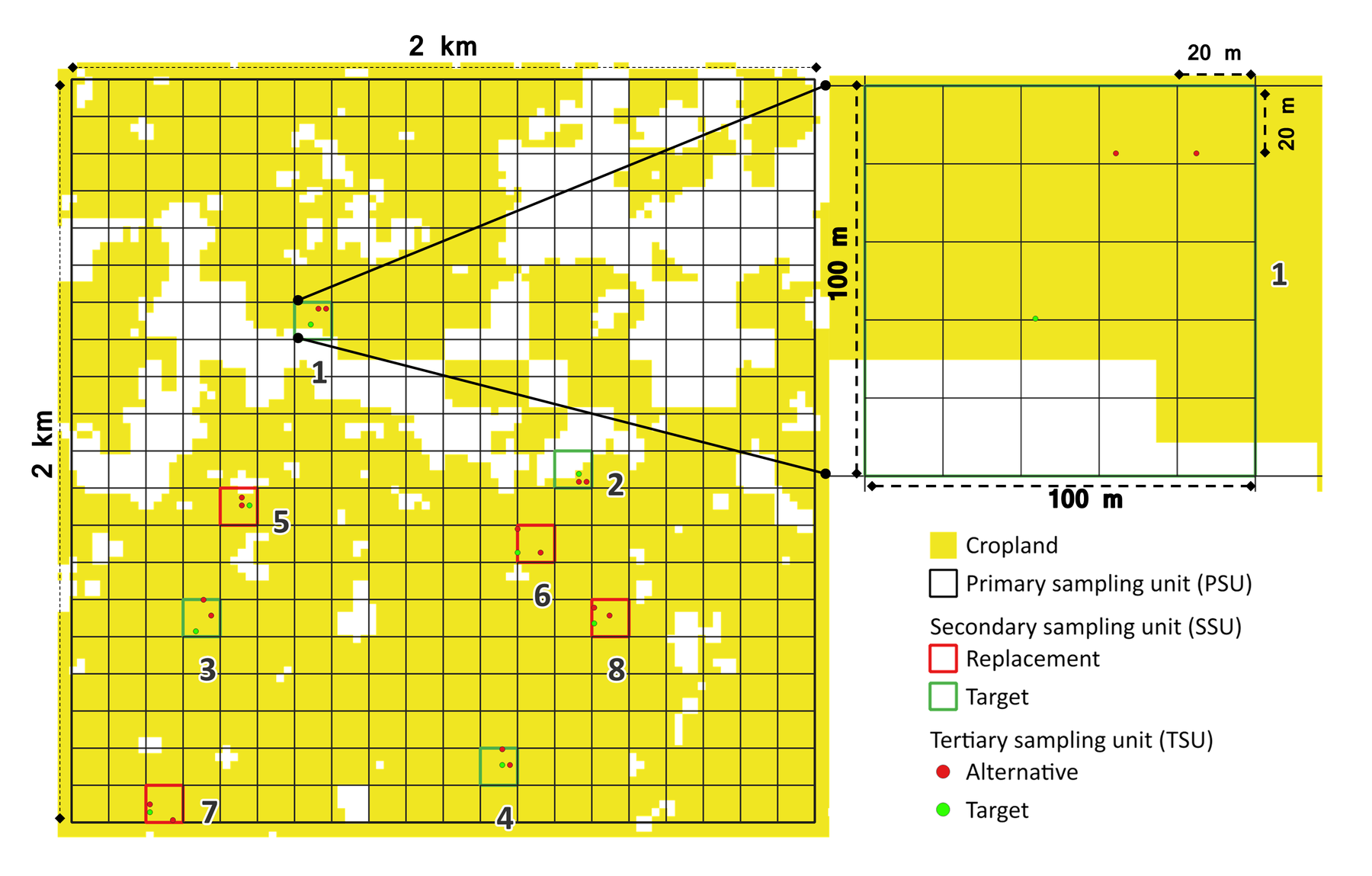
Figure 2.1: Example of a primary sampling unit with eight secondary sampling units, each containing three tertiary sampling units. Target units or points are in green, and replacements are in red.

2.3.3.1 PSU Selection Process

The process of selecting the PSUs is summarized as follows:

Step 1: Create 2km × 2km Grid (Figure 2.2) - A 2km × 2km grid covering the entire region of interest (ROI) is created - This grid serves as the foundational structure for stratification and spatial analysis

Step 2: Overlay Land Use and Protected Areas (Figure 2.3) - Land use and land cover (LULC) mask layer identifying cropland, forest, or grassland is overlaid - Protected area boundaries are incorporated - Grid cells where cropland, forest, or grassland cover more than 10% (or specified percentage) are retained - This ensures that only PSUs containing target land uses are selected

Step 3: Apply Covariate Space Coverage (Figure 2.4) - PSUs are selected through CSC sampling using 85 environmental covariates - Covariates are resampled to 250m resolution - Principal Component Analysis (PCA) transforms covariates into PC layers - PC layers accounting for up to 99% of variance are retained - PC layers are upscaled to 2km × 2km resolution

Step 4: Determine Optimal Sample Size - Optimal number of PSUs determined using divergence metrics - Kullback-Leibler Divergence (KLD) quantifies how well sampled data represents full environmental covariate space - Unlike Jensen-Shannon methods, KLD does not overestimate optimal sample size (Saurette et al., 2023)

Step 5: Perform K-means Clustering - K-means clustering creates homogeneous clusters (strata) - Number of clusters equals total number of PSUs to be sampled - Legacy point data can be incorporated (clusters fixed at legacy locations) - Mean Squared Shortest Distance (MSSD) in covariate space is calculated - Process repeated 10 times, retaining trial with minimum MSSD

Step 6: Select Target and Replacement PSUs (Figure 2.5) - PSUs allocated by minimizing MSSD within environmental covariate space - Output: N PSUs where N equals total number of samples - Replacement PSUs calculated by randomly selecting grid cells within same cluster class

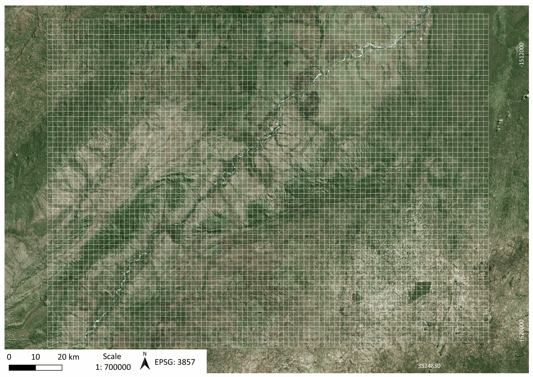
Figure 2.2: A 2×2 km grid is created across the region of interest.

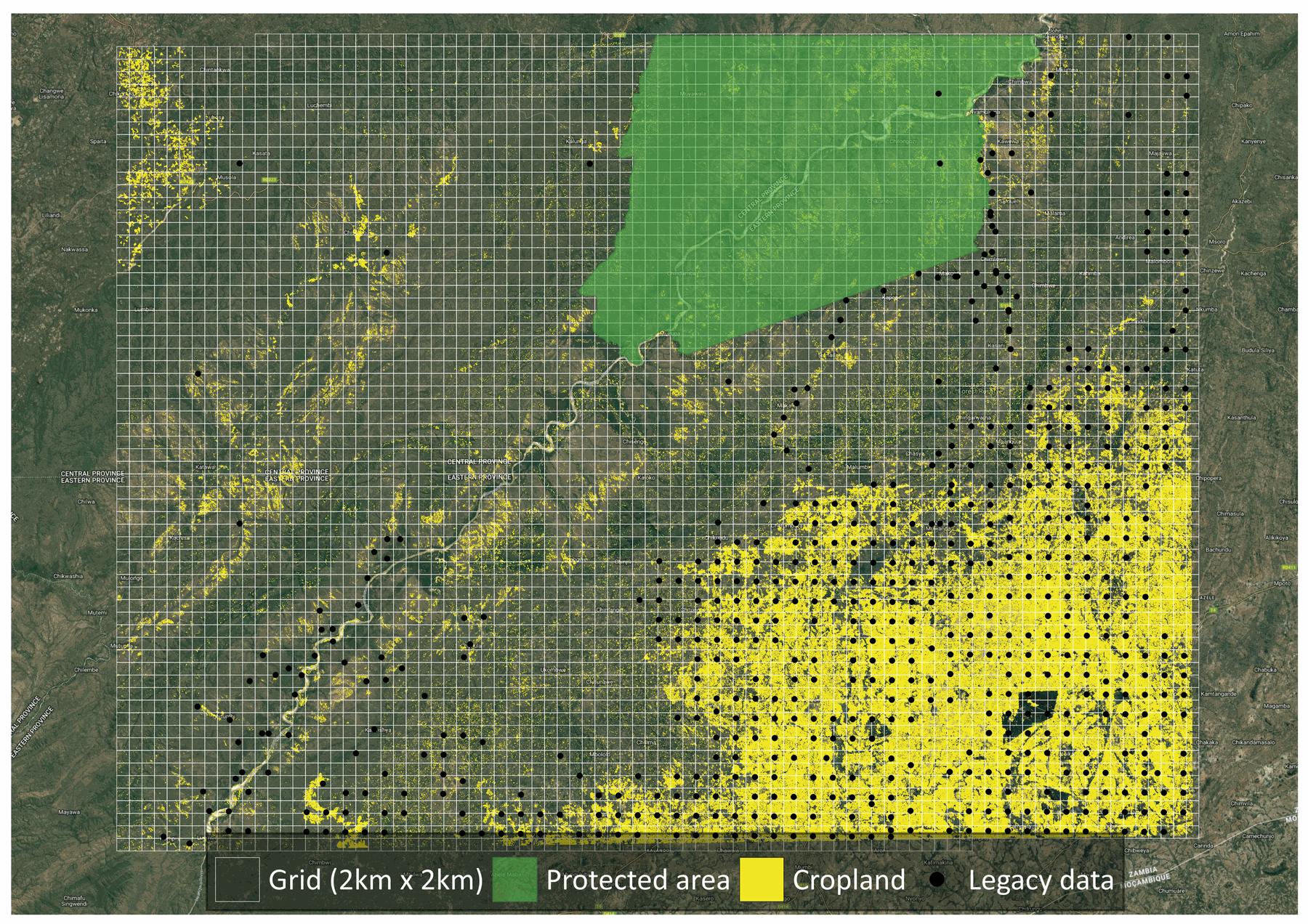
Figure 2.3: The grid is overlaid with legacy point data, crop layer data and protected area boundaries.

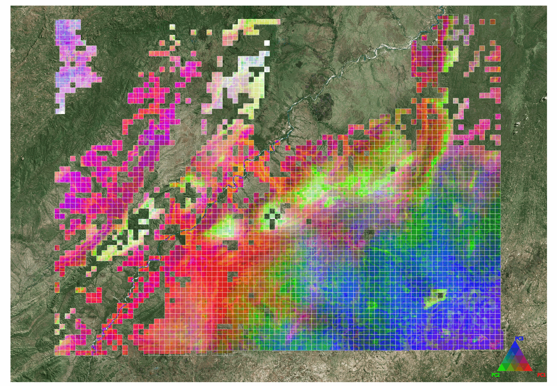
Figure 2.4: PSUs located in non-protected areas and containing more than 10% or any specified percentage of crop coverage are selected. The Covariate Space Coverage sampling method, incorporating 85 environmental covariates, is applied to identify target and replacement PSUs.

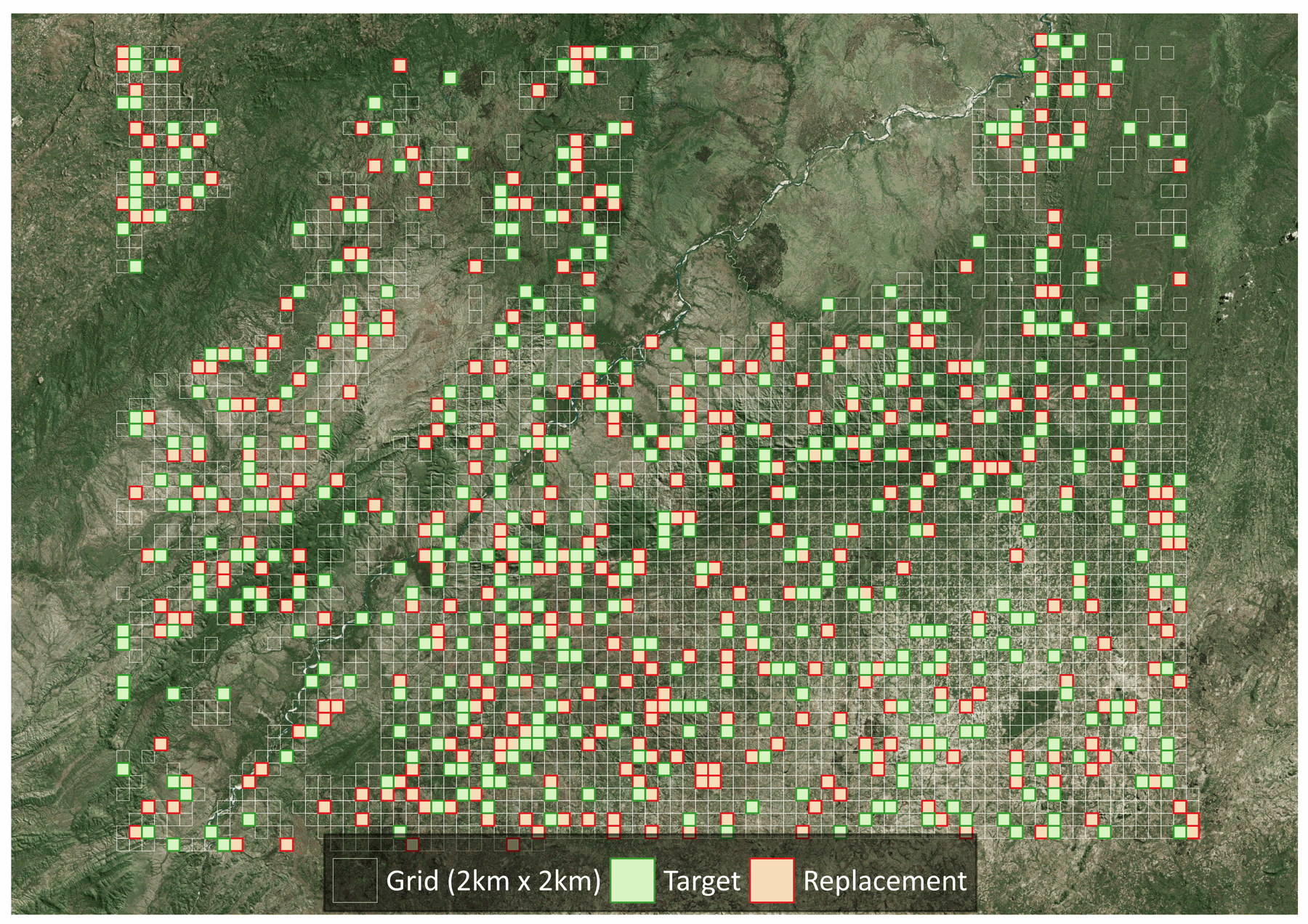
Figure 2.5: The selected target and replacement PSUs.

2.3.3.2 SSU and TSU Selection Process

Stage 2: Secondary Sampling Units (SSUs)

The second stage involves selecting SSUs using Covariate Space Coverage Sampling (CSCS) based on 24 high-resolution environmental covariates. Each SSU represents a 100m × 100m (1 hectare) area divided into 25 regular sampling plots of 20m × 20m (Figure 2.6).

Selection scheme: - 8 SSUs selected from each PSU - 4 target SSUs (1-4): where samples will be collected
- 4 replacement SSUs (5-8): pre-identified substitutes - Replacement SSUs directly linked to targets (one-to-one basis): - SSU 5 replaces SSU 1 - SSU 6 replaces SSU 2 - SSU 7 replaces SSU 3 - SSU 8 replaces SSU 4

If all SSUs within a target PSU are exhausted, missing SSUs must be selected from the designated PSU replacement. The designated PSU replacements were selected with the same spatial variability as their PSU targets.

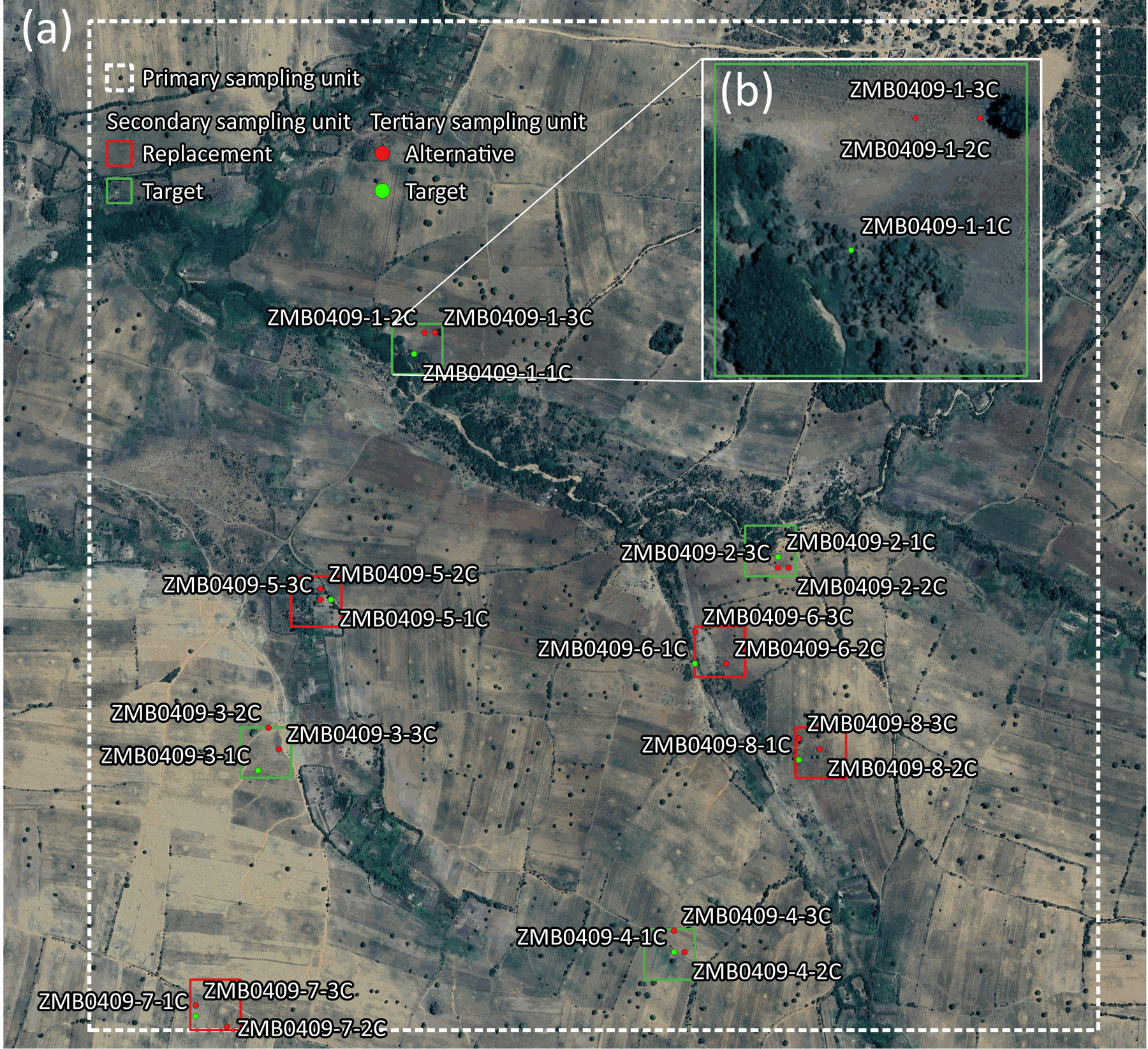
Figure 2.6: Single primary sampling unit displaying secondary sampling units (a), and a zoomed-in view of a secondary sampling unit with tertiary sampling units (b).

Stage 3: Tertiary Sampling Units (TSUs)

The third and final stage involves selecting TSUs using simple random sampling without replacement. Each SSU contains 25 possible TSUs of 20m × 20m, corresponding to the pixel size of the crop raster layer.

Selection scheme: - 3 TSUs per SSU: - 1 target TSU (primary sampling location) - 2 replacement TSUs (alternatives) - If a TSU is unsuitable, any replacement can be used - If all TSUs within an SSU are unsuitable, the entire SSU is rejected

Soil sampling protocol: - Sampling conducted strictly at designated TSU locations - Maximum shift: 10 metres from defined coordinates

2.3.3.3 Site Identification System

The final site ID is an alphanumeric identifier structured as follows (Figure 2.7):

Format: AAA####-#-#X

Where: - AAA = Three-letter country ISO code (e.g., KEN for Kenya) - #### = Primary Sampling Unit number (zero-padded, e.g., 0001) - First # = Secondary Sampling Unit number (1-8) - Second # = Tertiary Sampling Unit number (1-3) - X = Land use type code: - C = Cropland - G = Grassland - F = Forest

Example: KEN0001-1-1C - Country: Kenya - PSU: 1 - SSU: 1 (target) - TSU: 1 (target) - Land use: Cropland

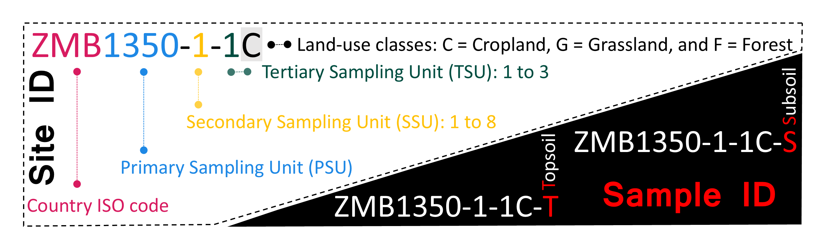
Figure 2.7: Deciphering the site identification.

2.4 Tutorial using R

This tutorial is designed for users with a basic understanding of R programming and provides a comprehensive guide to implementing a soil sampling design for soil monitoring and mapping. All scripts and data are available in the SoilFER Training Resources GitHub repository, specifically within the scripts and initial data directories.

💡 Note: Ensure you have the tinytex, knitr, rmarkdown, and rstudioapi R packages installed to successfully run and render R Markdown documents before running this script. Additionally, install tinytex by running tinytex::install_tinytex() to enable LaTeX support for PDF generation.

2.4.1 Setting up the environment

First, set the working directory to the location of your R script. This ensures that all paths in the script are relative to the script’s location.

setwd(dirname(rstudioapi::getActiveDocumentContext()$path))
setwd("../") # Move wd down to the main folder
getwd()

2.4.2 Install required libraries

The script uses several R libraries, each serving a specific purpose (Table 2.5).

Table 2.5: Summary of required R libraries and their purposes for SoilFER sampling design

Package	Purpose
sp	Spatial data classes
terra	Raster data manipulation
raster	Legacy raster support
sf	Simple features (vector data)
sgsR	Spatial sampling
entropy	Entropy calculations
tripack	Triangulation
tibble	Data frames
manipulate	Interactive plotting
dplyr	Data manipulation
synoptReg	PCA for rasters
doSNOW	Parallel processing
Rfast	Fast R functions
fields	Distance calculations
ggplot2	Visualization
rassta	Terrain analysis

Some libraries might need to be installed from GitHub. Uncomment and run the lines below if needed:

# Install synoptReg package from GitHub
# install.packages("remotes") # Install remotes if not installed
# remotes::install_github("lemuscanovas/synoptReg")

packages <- c("sp", "terra", "raster", "sf", "sgsR", "entropy", 
              "tripack", "tibble", "manipulate", "dplyr", "synoptReg", 
              "doSNOW", "Rfast", "fields", "ggplot2", "rassta")

invisible(lapply(packages, library, character.only = TRUE))

rm(packages)

Alternative method: In RStudio, use the Packages tab in the bottom-right pane → click Install → type package name → ensure “Install dependencies” is checked → click Install.

2.4.3 Define variables and parameters

Several variables and parameters must be defined to establish a consistent framework for the script.

2.4.3.1 Country ISO code

ISO.code <- "KANSAS"  

💡 Note: Use the Alpha-3 ISO code for your country of interest.

2.4.3.2 Land-use type

The SoilFER project focuses on three primary land-use types: croplands (85%), grasslands (10%), and forests (5%).

landuse <- "crops"  # Options: "crops", "grassland", "forest"

2.4.3.3 File paths

# Path to data folders
raster.path <- "data/rasters/"
shp.path <- "data/shapes/"
other.path <- "data/other/"
landuse_dir <- paste0("data/results/", landuse, "/")
   
# Check if the directory exists; if not, create it
dir.create(other.path, showWarnings = FALSE, recursive = TRUE)
dir.create("results",  showWarnings = FALSE, recursive = TRUE)
if (!file.exists(landuse_dir)) dir.create(landuse_dir)
results.path <- landuse_dir

2.4.3.4 Coordinate reference system

epsg <- "EPSG:3857"  # NAD27 UTM Zone 14N – adjust for your study area
# Find your CRS at: https://epsg.io/

2.4.3.5 Sample size calculation

# Manual set-up
nsamples <- 300  # Total sampling sites
share <- 0.80    # 80% for this land use (croplands)
nsites <- nsamples * share  # Final number of sites

💡 Note: Optimal sample size (N) is calculated statistically later.

2.4.3.6 Sampling unit definitions

# Define PSU and SSU sizes 
psu_size <- 2000   # PSU: 2km × 2 km
ssu_size <- 100    # SSU: 100m × 100m = 1 ha

# Define number of target and alternative SSUs at each PSU
num_primary_ssus     <- 4   # Target SSUs per PSU
num_alternative_ssus <- 4   # Replacement SSUs per PSU
number_TSUs          <- 3   # TSU points per SSU

2.4.3.7 Algorithm parameters

iterations   <- 10   # K-means random starts
percent_crop <- 20   # Minimum crop coverage for PSU selection (%)

2.4.4 Custom functions

2.4.4.1 Covariate Space Coverage (CSIS)

The CSIS function is the backbone of clustering sampling units in covariate space. It ensures optimal distribution while considering any fixed legacy data.

How it works:

1. Input parameters:
   • fixed: Preselected (legacy) sampling points
   • nsup: Number of additional (new) sampling points to select
   • nstarts: Number of random starting points for clustering
   • mygrd: Grid of covariate data for ROI
2. Workflow:
   • Extract fixed points and exclude from grid
   • Randomly initialize new sampling points
   • Combine fixed and new centers
   • Compute distances and assign points to nearest cluster
   • Update cluster centers iteratively until convergence
   • Calculate Mean Squared Shortest Distance (MSSSD)
   • Save best clustering result

## This function performs constrained k-means clustering
CSIS <- function(fixed, nsup, nstarts, mygrd) {
  # Args:
  #   fixed: Data frame of fixed legacy points
  #   nsup: Number of supplementary points to select
  #   nstarts: Number of random starts for optimization
  #   mygrd: Grid of all potential sampling locations
  
  n_fix <- nrow(fixed)
  p <- ncol(mygrd)
  units <- fixed$units
  mygrd_minfx <- mygrd[-units, ]
  MSSSD_cur <- NA
  
  for (s in 1:nstarts) {
    units <- sample(nrow(mygrd_minfx), nsup)
    centers_sup <- mygrd_minfx[units, ]
    centers <- rbind(fixed[, names(mygrd)], centers_sup)
    
    repeat {
      D <- rdist(x1 = centers, x2 = mygrd)
      cluster <- apply(X = D, MARGIN = 2, FUN = which.min) %>% as.factor(.)
      centers_cur <- centers
      
      for (i in 1:p) {
        centers[, i] <- tapply(mygrd[, i], INDEX = cluster, FUN = mean)
      }
      
      # Restore fixed centers (legacy data points don't move)
      centers[1:n_fix, ] <- centers_cur[1:n_fix, ]
      
      # Check convergence
      sumd <- diag(rdist(x1 = centers, x2 = centers_cur)) %>% sum(.)
      if (sumd < 1E-12) {
        D <- rdist(x1 = centers, x2 = mygrd)
        Dmin <- apply(X = D, MARGIN = 2, FUN = min)
        MSSSD <- mean(Dmin^2)
        
        if (s == 1 | MSSSD < MSSSD_cur) {
          centers_best <- centers
          clusters_best <- cluster
          MSSSD_cur <- MSSSD
        }
        break
      }
    }
    print(paste0(s," out of ",nstarts))
  }
  list(centers = centers_best, cluster = clusters_best)
}

💡 Note: This function creates spatially balanced sampling designs by considering existing sampling points and covariate distributions.

2.4.4.2 K-means with progress reporting

kmeans_with_progress <- function(data, centers, iter.max = 10000, nstart = 100) {
  # Provides visual feedback during long k-means operations
  best_result <- NULL
  best_totss <- Inf
  
  cat("Running k-means clustering with", nstart, "random starts...\n")
  
  for (s in 1:nstart) {
    result <- kmeans(data, centers = centers, iter.max = iter.max, nstart = 1)
    
    if (result$tot.withinss < best_totss) {
      best_result <- result
      best_totss <- result$tot.withinss
    }
    
    print(paste0(s, " out of ", nstart))
  }
  
  cat("Best tot.withinss:", best_totss, "\n")
  return(best_result)
}

2.4.4.3 TSU generation

This function generates TSUs within SSUs, ensuring random distribution while respecting land-use constraints.

## This function creates random point samples within each SSU polygon
generate_tsu_points_within_ssu <- function(ssu, number_TSUs, index, ssu_type, crops) {
  # Args:
  #   ssu: Single SSU polygon (sf object)
  #   number_TSUs: Number of points to generate
  #   index: SSU identifier
  #   ssu_type: "Target" or "Replacement"
  #   crops: Crop mask raster (20m resolution)
  
  ssu_vect <- vect(ssu)
  
  # Validate geometry
  if (is.null(ssu_vect) || nrow(ssu_vect) == 0 || is.na(ext(ssu_vect))) {
    warning(paste("SSU", index, "has invalid geometry. Skipping TSU generation."))
    return(NULL)
  }
  
  # Clip crop raster to SSU
  clipped_lu <- try(crop(crops, ssu_vect), silent = TRUE)
  if (inherits(clipped_lu, "try-error") || is.null(clipped_lu)) {
    warning(paste("SSU", index, "could not crop land use raster. Skipping."))
    return(NULL)
  }
  
  # Sample points (tries two methods)
  sampled_points <- try(sample_srs(clipped_lu, nSamp = number_TSUs), silent = TRUE)
  if (inherits(sampled_points, "try-error") || is.null(sampled_points) || nrow(sampled_points) == 0) {
    sampled_points <- try(spatSample(clipped_lu, size = number_TSUs, na.rm = TRUE, method = "random"), silent = TRUE)
  }
  
  if (inherits(sampled_points, "try-error") || is.null(sampled_points) || nrow(sampled_points) == 0) {
    warning(paste("SSU", index, "failed to generate TSUs. Skipping."))
    return(NULL)
  }
  
  # Add metadata
  sampled_points$PSU_ID <- selected_psu$ID
  sampled_points$SSU_ID <- index
  sampled_points$TSU_ID <- seq_len(nrow(sampled_points))
  sampled_points$SSU_Type <- ssu_type
  sampled_points$TSU_Name <- paste0(sampled_points$PSU_ID, ".", index, ".", seq_len(nrow(sampled_points)))
  
  return(sampled_points)
}

2.4.5 Load country boundaries and legacy data

Load and transform country boundaries and legacy soil data to the desired CRS:

# Purpose: Import study area boundaries and existing soil sample locations

# Load country/region boundaries
country_boundaries <- file.path(paste0(shp.path,"roi_kansas_us_epsg_4326.shp"))
country_boundaries <- sf::st_read(country_boundaries, quiet=TRUE)

# Reproject if necessary
if(crs(country_boundaries)!=epsg){
  country_boundaries <- country_boundaries %>%
    st_as_sf() %>% sf::st_transform(crs=epsg)
}

# Load legacy soil data (optional - existing sample points)
legacy <- file.path(paste0(shp.path,"soil_legacy_data_kansas_epsg_4326.shp"))

if(file.exists(legacy)){
  legacy <- sf::st_read(legacy, quiet=TRUE)
  if(crs(legacy)!=epsg){
    legacy <- legacy %>% sf::st_transform(crs=epsg)
  }
} else {
  rm(legacy)  # Remove if doesn't exist
} 

# Clean legacy data
if(exists("legacy")){
  legacy <- dplyr::select(legacy, geometry)
  legacy <- legacy[!duplicated(st_geometry(legacy)), ]  # Remove duplicates
}

💡 Note: Always verify that all geospatial datasets use the same CRS before performing spatial operations. Misaligned CRSs can lead to incorrect analyses.

2.4.5.1 Visualize boundaries and legacy data

# Visualize boundaries and legacy points
ggplot() +
  geom_spatvector(data = country_boundaries, fill = NA, color = "black") +
  geom_spatvector(data = legacy, aes(geometry = geometry), size = 0.7, color = "red") +
  theme_minimal()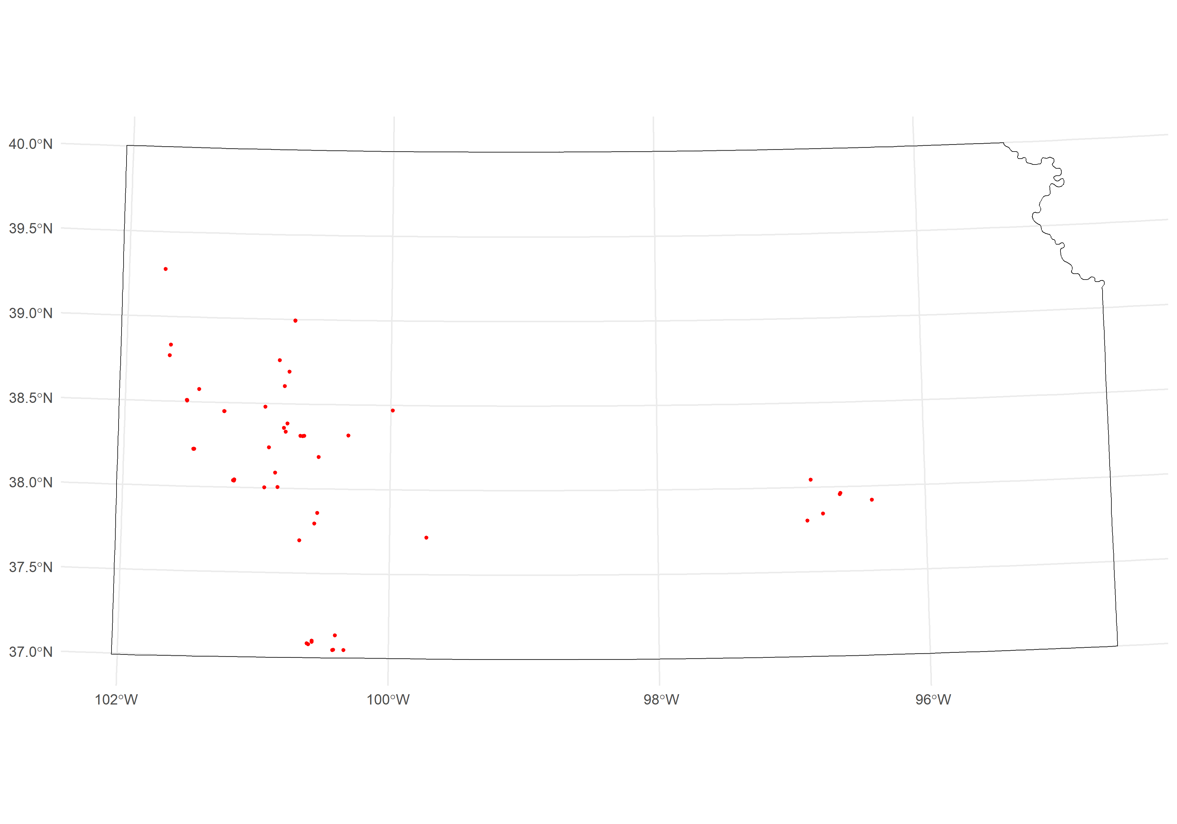

Figure 2.8: Grey rectangle outlines the region of interest, while red dots represent the geolocations of the legacy data points.

2.4.6 Load environmental covariates for PSUs

In many sampling campaigns, not all areas within the country or region of interest are suitable for fieldwork. Protected areas may be legally restricted, steep terrain may be unsafe or inaccessible, and other constraints (e.g., water bodies, urban zones) can reduce the feasible sampling space. For this reason, SoilFER treats “exclusion layers” as optional inputs that refine the accessible area without changing the overall survey objective. When an exclusion layer is available, it is loaded, reprojected to the common CRS used in the project, and then converted into a mask that can be applied to the sampling universe. If a layer is not available, the script continues without it, ensuring that the workflow remains robust across countries with different data availability.

In addition to exclusion layers, ancillary datasets such as geology or geomorphology can be used for stratification. These layers do not exclude areas from sampling; instead, they provide categorical information that may help define strata or interpret spatial patterns during mapping and analysis.

2.4.6.1 Protected areas mask (exclude from sampling)

This chunk checks whether a protected-areas shapefile exists. If it does, the polygons are read, transformed to the project CRS if needed, dissolved into a single geometry, and then subtracted from the country boundary. The result is a “non-protected” mask representing areas where sampling is allowed.

# Protected areas (areas to EXCLUDE from sampling)
npa <- file.path(paste0(shp.path,"protected_areas_epsg_4326.shp"))

if(file.exists(npa)){
  npa <- sf::st_read(npa, quiet = FALSE)
  if(crs(npa)!=epsg){
    npa <- npa %>% sf::st_transform(crs = epsg)
  }
  npa <- sf::st_union(npa)
  npa <- sf::st_difference(country_boundaries, npa)  # Create "non-protected" mask
} else {
  rm(npa)
}

ggplot() +
  geom_sf(data = npa, fill = "grey90", color = "black", linewidth = 0.3) +
  coord_sf(datum = NA) +
  labs(title = "Accessible area mask (non-protected in grey)") +
  theme_minimal(base_size = 11)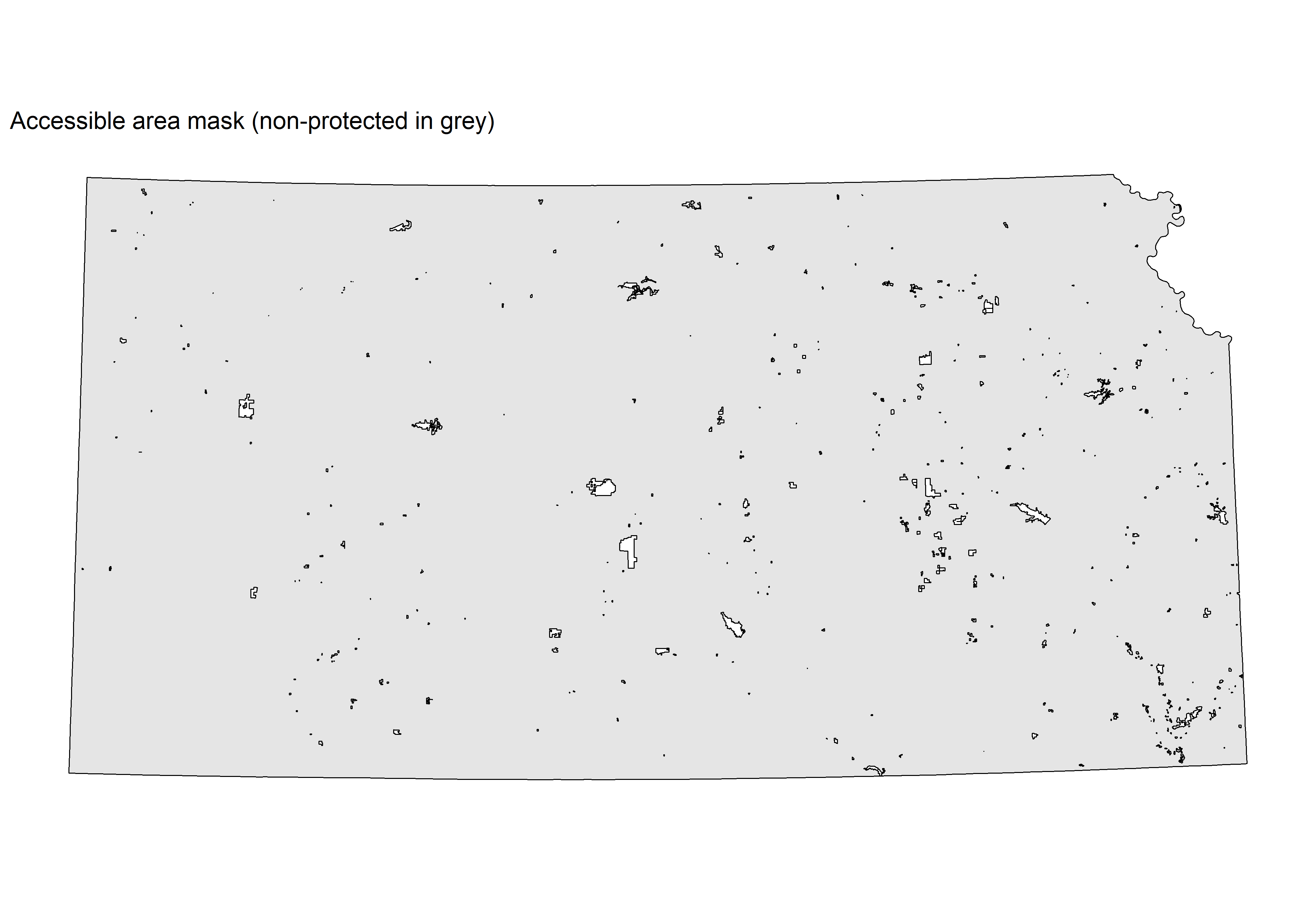

Figure 2.9: Protected areas (empty shapes)

2.4.6.2 Slope mask (exclude steep terrain)

This chunk checks whether a pre-processed binary slope raster exists. If it does, the raster is loaded, reprojected to the project CRS if needed, normalised to a strict binary mask (1/NA) by dividing by itself, and then clipped to the country boundary. The result is a raster where cells with value 1 represent accessible slopes and all excluded cells are NA. If the file is not found, the object is removed so downstream code knows no slope filter applies.

💡 Note: The slope mask must be prepared before running this script. In QGIS, use the Raster Calculator with the formula (“Slope@1” <= 30) * 1 to create a binary raster (1: accessible, 0: excluded), then use the Set Null tool to convert 0 to NA.
Threshold guidelines: gentle terrain 0-15%, moderate terrain 15-30% (typical field-work threshold), steep terrain > 30% (usually excluded).

slope <- file.path(paste0(raster.path,"slope_mask_epsg_4326.tif"))

if(file.exists(slope)){
  slope <- rast(slope)
  if(crs(slope)!=epsg){
    slope <- project(slope, epsg, method="near")
  }
  slope <- slope/slope  # Convert to binary mask
  slope <- terra::mask(slope, country_boundaries)
} else {
  rm(slope)
}

plot(slope,
     col = "#66c2a5",
     legend = FALSE,
     main = "Slope accessibility mask in green")

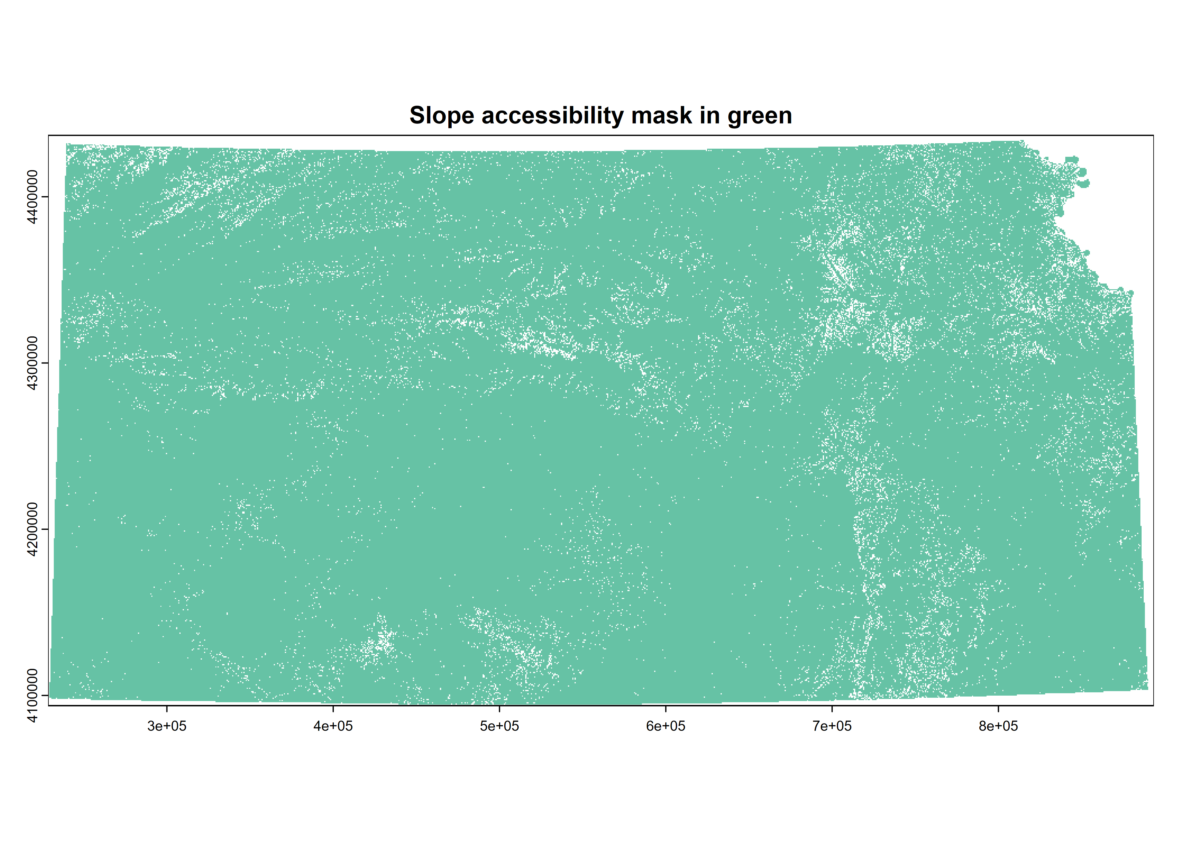
Figure 2.10: Slope accessibility areas

2.4.6.3 Ecoregions / Geology data (for stratification)

This chunk checks whether an ecoregions shapefile exists. If it does, the polygons are read, reprojected to the project CRS if needed, and a numeric GEO field is created by converting the ecoregion name column to a factor and then to an integer. This numeric encoding is required for rasterization and dummy-variable conversion in later steps. If the file is not found, the object is removed so downstream code knows no geology stratification applies.

💡 Note: For Kansas, ecoregion boundaries (US_L3NAME field) are used as a geology proxy. For other study areas, replace the shapefile path and update geo.classes to match the field name containing your geological or ecoregion classification. Any polygon layer with a categorical attribute can be used here.

# Geology data (for stratification) - If available
geo <- file.path(paste0(shp.path,"ecoregions_kansas_epsg_4326.shp"))
geo.classes <- "US_L3NAME"  # Field name for geology classes

if(file.exists(geo)){
  geo <- sf::st_read(geo, quiet=TRUE)
  if(crs(geo)!=epsg){
    geo <- geo %>% sf::st_transform(crs=epsg)
  }
  geo$GEO <- as.numeric(as.factor(geo[[geo.classes]]))
} else {
  rm(geo)
}

ggplot() +
  geom_sf(data = geo, aes(fill = US_L3NAME), color = "black", linewidth = 0.2) +
  labs(title = "Level III Ecoregions",
       fill = "Ecoregion (US_L3NAME)") +
  theme_minimal(base_size = 11) +
  theme(legend.position = "right")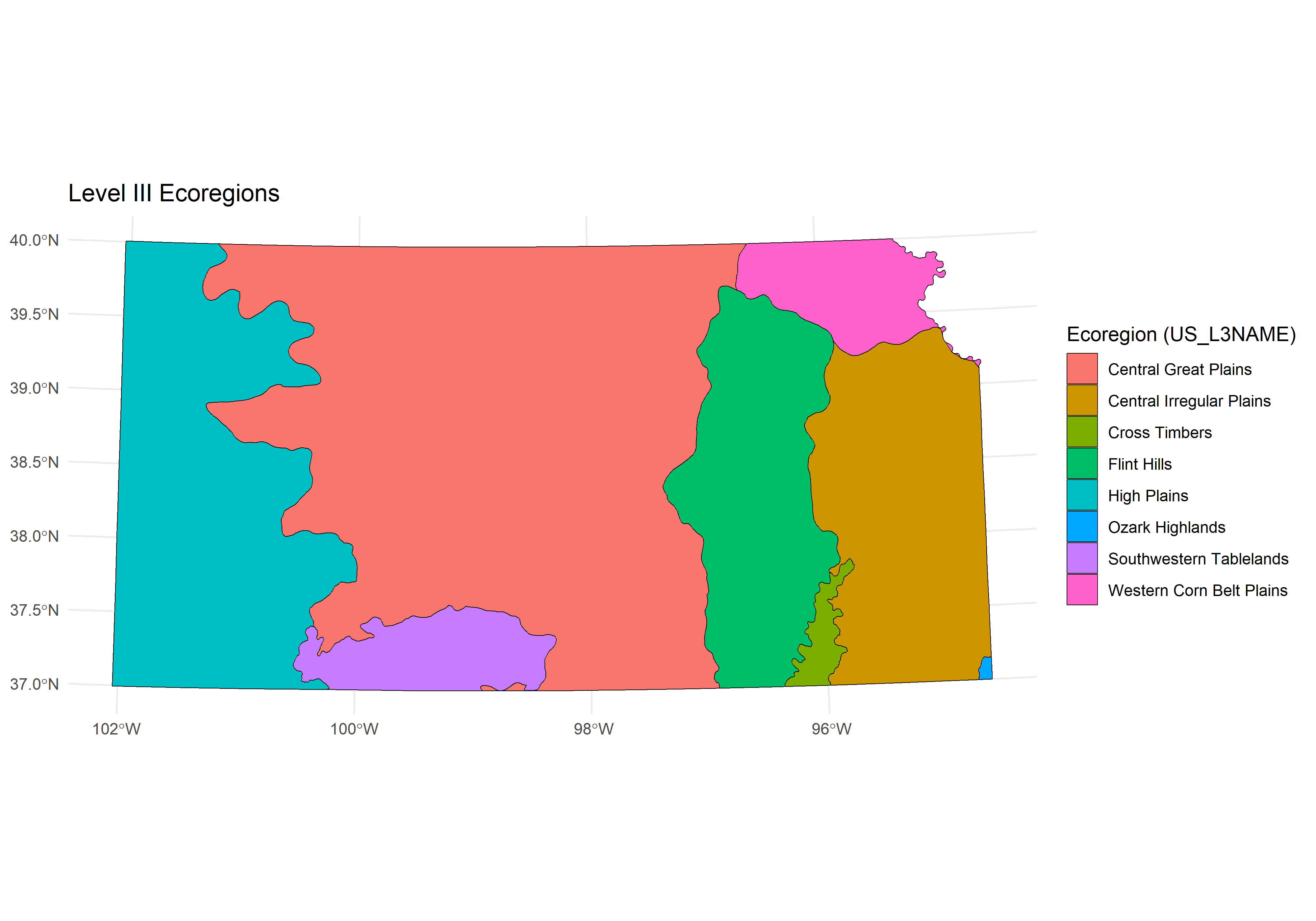

Figure 2.11: Ecoregions

2.4.6.4 Geomorphology data (for stratification)

This chunk checks whether a geomorphology file exists and handles two possible formats. If the file is a raster (.tif), it is loaded, renamed to GEOMORPH, and reprojected if needed. If it is a shapefile (.shp), it is read as a vector, reprojected if needed, and a numeric GEOMORPH field is created by encoding the class column as integers. In both cases, the result is clipped to the country boundary. If the file is not found, the object is removed so downstream code knows no geomorphology stratification applies.

💡 Note: For Kansas, the geomorphology raster is exported from Google Earth Engine (GEE_Exports/) using the Geomorphon landform classification. Both raster (.tif) and vector (.shp) formats are supported. Update the file path and geomorph.classes field name to match your dataset. If using a shapefile, ensure the classification column contains categorical landform labels that can be factorised into integer codes.

# Geomorphology data (for stratification) - if available
geomorph <- file.path(paste0(raster.path, "/GEE_Exports/Geomorphon_Landforms_KANSAS.tif"))
geomorph.classes <- "Class"  # Field name for geomorphology classes (shapefile only)

if (file.exists(geomorph)) {
  file_extension <- tools::file_ext(geomorph)

  if (file_extension == "tif") {
    geomorph <- rast(geomorph)
    names(geomorph) <- "GEOMORPH"
    if (crs(geomorph) != epsg) {
      geomorph <- project(geomorph, epsg, method = "near")
    }
  } else if (file_extension == "shp") {
    geomorph <- sf::st_read(geomorph, quiet = TRUE)
    if (sf::st_crs(geomorph)$epsg != epsg) {
      geomorph <- sf::st_transform(geomorph, crs = epsg)
    }
    geomorph$GEOMORPH <- as.numeric(as.factor(geomorph[[geomorph.classes]]))  # Encode as integers
  }

  geomorph <- terra::mask(geomorph, country_boundaries)
} else {
  rm(geomorph)
}

# Create a class lookup table (Geomorpho90m / geomorphons)
geomorph_lut <- data.frame(
  value = 1:10,
  class = c(
    "Flat",
    "Peak / summit",
    "Ridge",
    "Shoulder",
    "Spur",
    "Slope",
    "Hollow",
    "Footslope",
    "Valley",
    "Pit / depression"
  )
)

# Semantically meaningful colors: warm tones for highs, cool tones for lows
geomorph_colors <- c(
  "Flat"             = "#F5F5DC",  # beige      – level ground
  "Peak / summit"    = "#8B0000",  # dark red   – highest points
  "Ridge"            = "#CD5C5C",  # indian red – elongated highs
  "Shoulder"         = "#D2691E",  # chocolate  – convex upper slopes
  "Spur"             = "#DAA520",  # goldenrod  – diverging slopes
  "Slope"            = "#6B8E23",  # olive      – planar slopes
  "Hollow"           = "#4682B4",  # steel blue – converging slopes
  "Footslope"        = "#5F9EA0",  # cadet blue – concave lower slopes
  "Valley"           = "#00008B",  # dark blue  – linear lows
  "Pit / depression" = "#191970"   # midnight   – lowest points
)

# Attach labels to the raster as categories
geomorph_cat <- as.factor(geomorph)
levels(geomorph_cat) <- list(data.frame(
  ID    = geomorph_lut$value,
  class = geomorph_lut$class
))

par(mar = c(3, 3, 4, 3), bg = "white")

plot(
  geomorph_cat,
  col  = geomorph_colors[levels(geomorph_cat)[[1]]$class],
  main = "Geomorphology",
  axes = FALSE,
  box = FALSE,
  plg = list(
    inset = c(0.02, 0.03),
    cex = 0.75,
    title = "Geomorphons",
    bty = "n"
  )
)

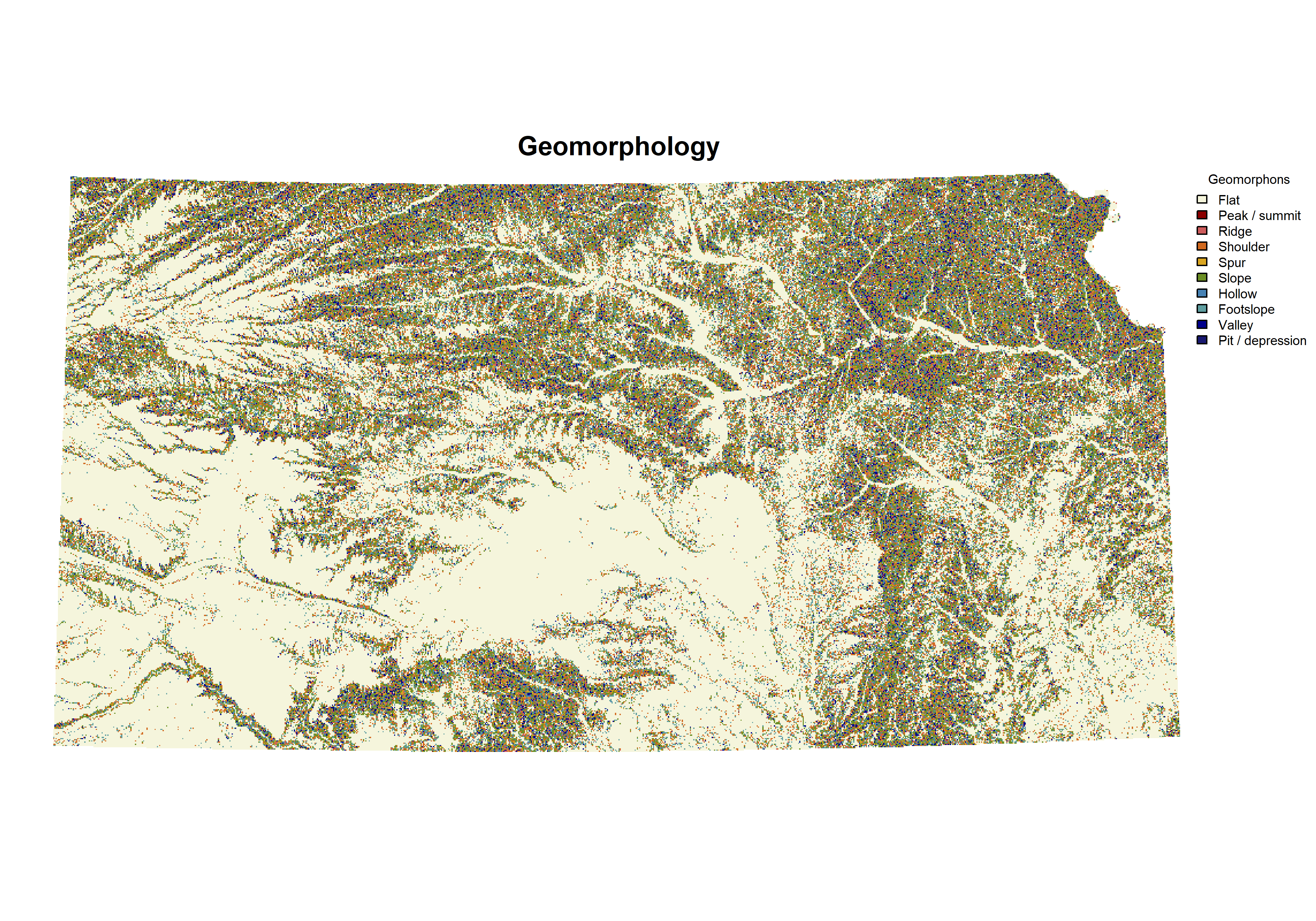
Figure 2.12: Geomorphology retrieved from GEE

2.4.6.5 Environmental covariates created/retrieved from previous Chapter

This section loads and prepares the environmental covariates used to delineate Primary Sampling Units (PSUs). These variables define the environmental space within which PSUs are distributed. First, the script locates and loads the environmental raster stack exported from Google Earth Engine (GEE). The raster file contains multiple environmental layers (e.g., climate, terrain, vegetation indices) at 250 m resolution. Second, the coordinate reference system (CRS) is checked. If the raster CRS does not match the project CRS (epsg), the data are reprojected using nearest-neighbour interpolation to preserve categorical values. Third, the raster stack is resampled to the PSU spatial resolution (2 km). A template raster is created using the desired PSU grid size (psu_size). The environmental layers are then aggregated to this coarser resolution using bilinear interpolation. This ensures that environmental variability is represented at the same spatial scale at which PSUs will be defined. The aggregation resolution must match the PSU size; otherwise, inconsistencies may arise between environmental stratification and sampling unit geometry. Finally, the raster stack is masked to the country boundary, ensuring that environmental data is retained only within the region of interest.

# Purpose: Load environmental data at 2km resolution for PSU selection from GEE code
# Note: These covariates determine WHERE PSUs are placed

cov.dat <- list.files(paste0(raster.path, "GEE_Exports/"), 
                      pattern = "Environmental_Covariates_250m_KANSAS.tif$",  
                      recursive = TRUE, full.names = TRUE)
cov.dat <- terra::rast(cov.dat)

# Reproject if necessary
if(crs(cov.dat)!=epsg){
  cov.dat <- terra::project(cov.dat, epsg, method="near")
}

# Resample to PSU resolution (2km)
# IMPORTANT: This aggregation must match your PSU size
psu_size_template <- rast(ext(cov.dat), resolution = psu_size, crs = crs(cov.dat))
cov.dat <- resample(cov.dat, psu_size_template, method = "bilinear")
cov.dat <- terra::mask(cov.dat, country_boundaries)

Table 2.6: Environmental covariates used for Primary Sampling Unit (PSU) delineation.

	Category	Variable
1	Climate (CHELSA)	bio1
2	Climate (CHELSA)	bio5
3	Climate (CHELSA)	bio6
4	Climate (CHELSA)	bio12
5	Climate (CHELSA)	bio13
6	Climate (CHELSA)	bio14
7	Climate (CHELSA)	bio16
8	Climate (CHELSA)	bio17
9	Energy & Water Balance	ngd10
10	Energy & Water Balance	pet_penman_max
11	Energy & Water Balance	pet_penman_mean
12	Energy & Water Balance	pet_penman_min
13	Energy & Water Balance	pet_penman_range
14	Energy & Water Balance	sfcWind_max
15	Energy & Water Balance	sfcWind_mean
16	Energy & Water Balance	sfcWind_range
17	Vegetation Indices (MODIS)	fpar_*_mean/sd
18	Vegetation Indices (MODIS)	lstd_*_mean/sd
19	Vegetation Indices (MODIS)	ndlst_*_mean/sd
20	Vegetation Indices (MODIS)	ndvi_*_mean/sd
21	Vegetation Indices (MODIS)	snow_cover
22	Vegetation Indices (MODIS)	swir_060708_500m_mean
41	Land Cover	crops
42	Land Cover	flooded_vegetation
43	Land Cover	grass
44	Land Cover	shrub_and_scrub
45	Land Cover	trees
47	Terrain Derivatives (DTM)	dtm_elevation_250m
48	Terrain Derivatives (DTM)	dtm_slope_250m
49	Terrain Derivatives (DTM)	dtm_tpi_250m
50	Terrain Derivatives (DTM)	dtm_twi_500m
51	Terrain Derivatives (DTM)	dtm_curvature_250m
52	Terrain Derivatives (DTM)	dtm_upslopecurvature_250m
53	Terrain Derivatives (DTM)	dtm_downslopecurvature_250m
54	Terrain Derivatives (DTM)	dtm_vbf_250m
55	Terrain Derivatives (DTM)	dtm_mrn_250m
56	Terrain Derivatives (DTM)	dtm_dvm_250m
57	Terrain Derivatives (DTM)	dtm_dvm2_250m

💡 Note: Initial number of environmental covariates is 66.

2.4.6.6 Load and process soil-climate data (Newhall)

The Newhall soil-climate dataset provides categorical (i.e., regime classes) and continuous variables describing soil temperature and moisture regimes. This section loads the Newhall raster, ensures it matches the project CRS, removes layers that are not required, and then harmonises all remaining layers to the same grid as the environmental covariates (cov.dat). Categorical layers are resampled using nearest-neighbour interpolation to preserve class identities, whereas continuous layers can be resampled with default interpolation.

# Load and process soil climate data
newhall <- list.files(raster.path, pattern = "newhall.tif$", recursive = TRUE, full.names = TRUE)
newhall <- terra::rast(newhall)

if(crs(newhall)!=epsg){
  newhall <- terra::project(newhall, epsg, method="near")
}

# Remove unnecessary layers
newhall$regimeSubdivision1 <- NULL
newhall$regimeSubdivision2 <- NULL

# Process categorical variables (preserve factor levels)
temperatureRegime <- project(newhall$temperatureRegime, cov.dat, method = "near")
moistureRegime <- project(newhall$moistureRegime, cov.dat, method = "near")

newhall$temperatureRegime <- NULL
newhall$moistureRegime <- NULL
newhall <- terra::resample(newhall, cov.dat)

2.4.6.7 Convert soil-climate regimes to dummy variables

The Newhall soil-climate dataset includes categorical variables describing soil temperature and moisture regimes. Since these are nominal classes (e.g., mesic, thermic, ustic), they cannot be directly used in most statistical or machine-learning models. To incorporate them as predictors in the PSU selection workflow, each regime class is converted into a set of binary (dummy) variables. Each dummy layer represents the presence (1) or absence (0) of a specific regime class.

# Convert to dummy variables (one column per category)
temperatureRegime <- as.factor(temperatureRegime)
temperatureRegime <- dummies(ca.rast = temperatureRegime, preval = 1, absval = 0)
moistureRegime <- as.factor(moistureRegime)
moistureRegime <- dummies(ca.rast = moistureRegime, preval = 1, absval = 0)

2.4.6.8 Integrating all layers and finalising the Covariate Stack

At this stage, all continuous and categorical environmental predictors are combined into a single covariate stack (cov.dat). This stack defines the environmental feature space used for PSU placement. Optional stratification layers such as geology and geomorphology can be included when available. Because these layers are categorical, they are first rasterised to the covariate grid and then converted to dummy variables (one binary layer per class). Before merging, all optional layers are checked and harmonised to ensure they match the covariate stack in extent and resolution. Finally, the complete stack is cropped and masked to the study boundary and written to disk for reuse.

# Merge all covariates
cov.dat <- c(cov.dat, newhall, temperatureRegime, moistureRegime)

# Add geology if available
if(exists("geo")){
  geo <- rasterize(as(geo,"SpatVector"), cov.dat, field="GEO")
  geo <- dummies(ca.rast = geo$GEO, preval = 1, absval = 0)
  cov.dat <- c(cov.dat, geo)
}

# Add geomorphology if available
if (exists("geomorph")) {
  if (!inherits(geomorph, "SpatRaster")) {
    geomorph <- rasterize(as(geomorph, "SpatVector"), cov.dat, field = "GEOMORPH")
  }
  geomorph <- dummies(ca.rast = geomorph$GEOMORPH, preval = 1, absval = 0)
  
  # Ensure matching extents
  if (!identical(ext(cov.dat), ext(geomorph))) {
    geomorph <- extend(geomorph, cov.dat)
  }
  if (!all(res(cov.dat) == res(geomorph))) {
    geomorph <- resample(geomorph, cov.dat, method = "near")
  }
  
  cov.dat <- c(cov.dat, geomorph)
}

# Clean up
rm(newhall, geomorph)
gc()

# Crop to study area
cov.dat <- crop(cov.dat, country_boundaries, mask=TRUE, overwrite=TRUE)
## Saving the covariate stack if R clashes
writeRaster(cov.dat, paste0(raster.path,"cov_dat_stack_psus.tif"), overwrite=TRUE)

# Reload if needed
# cov.dat <- rast(paste0(raster.path, "cov_dat_stack_psus.tif"))

Table 2.7: Summary of environmental covariates included in the PSU selection stack (2 km resolution).

Category	Description	Number of layers
Climate (CHELSA bioclim)	Temperature and precipitation bioclimatic variables (bio1–bio17)	8
Energy & Atmospheric Variables	Growing degree days, PET, wind statistics	8
Vegetation Indices (MODIS seasonal)	FPAR, LST day/night, NDVI (seasonal mean and SD)	32
Land Cover	Fractional land cover classes (crops, trees, grass, etc.)	6
Terrain Derivatives (DTM)	Elevation, slope, curvature, TPI, TWI, VBF and derivatives	12
Soil Climate (Newhall continuous)	Water balance and moisture/temperature regime metrics	15
Soil Climate Regimes (Dummy variables)	Binary layers representing temperature and moisture regime classes	6
Geology (Dummy variables)	Binary layers representing geology/ecoregion classes	8
Geomorphology (Dummy variables)	Binary layers representing geomorphon landform classes	10

💡 Note: Stacking is the process of combining multiple spatial data layers (raster datasets) into a single multi-layer object. This is useful when multiple variables need to be analysed together. The final dataset comprises 85 environmental covariates, which expand to 105 raster layers after converting categorical variables into dummy (binary) layers.

2.4.7 Principal Component Analysis (PCA)

Environmental covariates such as satellite-derived spectral indices often exhibit strong inter-correlation because they are calculated from overlapping spectral bands and capture related biophysical properties (e.g., vegetation vigor, moisture content, surface reflectance characteristics). Such redundancy can inflate dimensionality and negatively affect clustering or classification procedures. To address this issue, a Principal Component Analysis (PCA) was applied to the standardised environmental covariate raster stack. Standardisation ensured that indices with different value ranges contributed equally to the analysis.

The PCA transforms correlated indices into orthogonal components representing dominant gradients across the landscape. These components summarise major patterns in surface reflectance and vegetation structure while removing multicollinearity among indices. Only the minimum number of principal components explaining more than 99% of the cumulative variance were retained. This threshold preserves nearly all information while substantially reducing data dimensionality and computational burden. The resulting principal component rasters were then exported for subsequent spatial clustering and landscape characterisation.

pca <- scale(cov.dat)
pca <- synoptReg::raster_pca(pca)  # Fast PCA for rasters

cov.dat <- pca$PCA

# Keep only components explaining 99% of variance
n_comps <- first(which(pca$summaryPCA[3,] > 0.99))
cov.dat <- pca$PCA[[1:n_comps]]

cat(sprintf("Using %d principal components (explaining >99%% variance)\n", n_comps))

# Save PCA results
writeRaster(cov.dat, paste0(results.path,"PCA_projected.tif"), overwrite=TRUE)
rm(pca)

# Reload for further processing
# Why this is useful:
#  - Previous sections (data loading, PCA) can take 30+ minutes
#  - If script crashes or needs modification, you can load here
#  - If the file exists in the folder from previous processing
# cov.dat <- rast(paste0(results.path,"PCA_projected.tif"))

# Reproject if necessary
if(crs(cov.dat)!=epsg){
  cov.dat <- terra::project(cov.dat, epsg, method="near")
}

# Visualising maps from PC1-PC3
# Consistent color scale across PC1–PC3
minmax_vals <- minmax(pca$PCA[[1:3]])
zlim_vals <- range(minmax_vals)

cols <- hcl.colors(100, "Blue-Red 3", rev = TRUE)

par(mfrow = c(1,3), mar = c(3,3,3,6))  # extra space for legend

plot(pca$PCA[[1]],
     col = cols,
     zlim = zlim_vals,
     main = "PC1",
     axes = FALSE,
     box = FALSE,
     plg = list(title = "PC value"))

plot(pca$PCA[[2]],
     col = cols,
     zlim = zlim_vals,
     axes = FALSE,
     box = FALSE,
     main = "PC2",
     plg = list(title = "PC value"))

plot(pca$PCA[[3]],
     col = cols,
     zlim = zlim_vals,
     main = "PC3",
     axes = FALSE,
     box = FALSE,
     plg = list(title = "PC value"))

# Plot cumulative variance
cum_var <- pca$summaryPCA["Cumulative", ]

plot(cum_var,
     type = "l",
     lwd = 2,
     xlab = "Principal Component",
     ylab = "Cumulative Variance Explained",
     main = "Cumulative Variance")

abline(h = 0.99, col = "red", lty = 2)

Figure 2.13: Spatial distribution of the first three principal components (PC1-PC3).

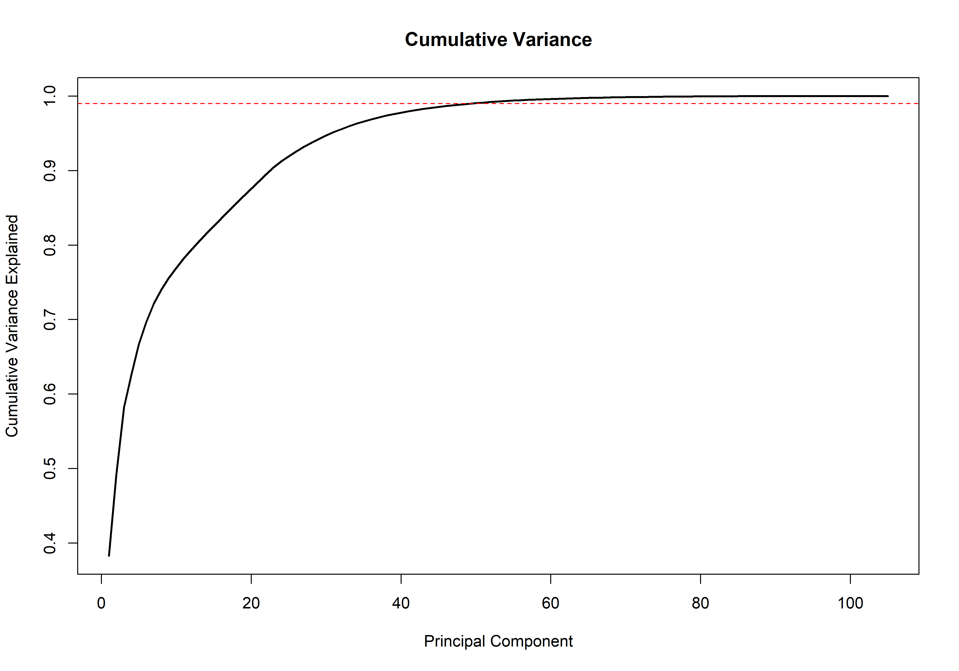
Figure 2.14: Cumulative variance explained.

2.4.8 Load and prepare land-use data

This section defines the sampling universe. That is the spatial area where sampling units are allowed to be placed. Two spatial resolutions are used:

• 20 m resolution: precise placement of Temporary Sampling Units (TSUs),

• 100 m resolution: filtering and aggregation for Primary Sampling Units (PSUs).

The cropland raster is loaded and converted to a binary mask where: 1 = cropland and NA = non-cropland. This ensures that subsequent sampling occurs only within agricultural areas.

# Define file path
landuse_file <- file.path(paste0(raster.path,"Cropland_Mask_KANSAS_merged.tif"))

# Load raster
crops <- rast(landuse_file)

# Convert to binary mask (1 = crop, NA = other)
crops <- crops / crops
names(crops) <- "lu"

The land-use raster is reprojected to match the coordinate reference system (CRS) used throughout the analysis. Nearest-neighbor interpolation is applied to preserve categorical values.

if(crs(crops) != epsg){
  crops <- terra::project(crops, epsg, method = "near")
}

# Display raster info
crops

Table 2.8: Metadata of the cropland mask raster.

Property	Value
Class	SpatRaster
Dimensions (rows, cols, layers)	21007 × 40716 × 1
Resolution (x, y)	16.32943 × 16.32943
Extent (xmin, xmax, ymin, ymax)	228591.3, 893460.4, 4093884, 4436916
Coordinate Reference System	NAD27 / UTM zone 14N (EPSG:26714)
Value Range	1–1 (binary mask)

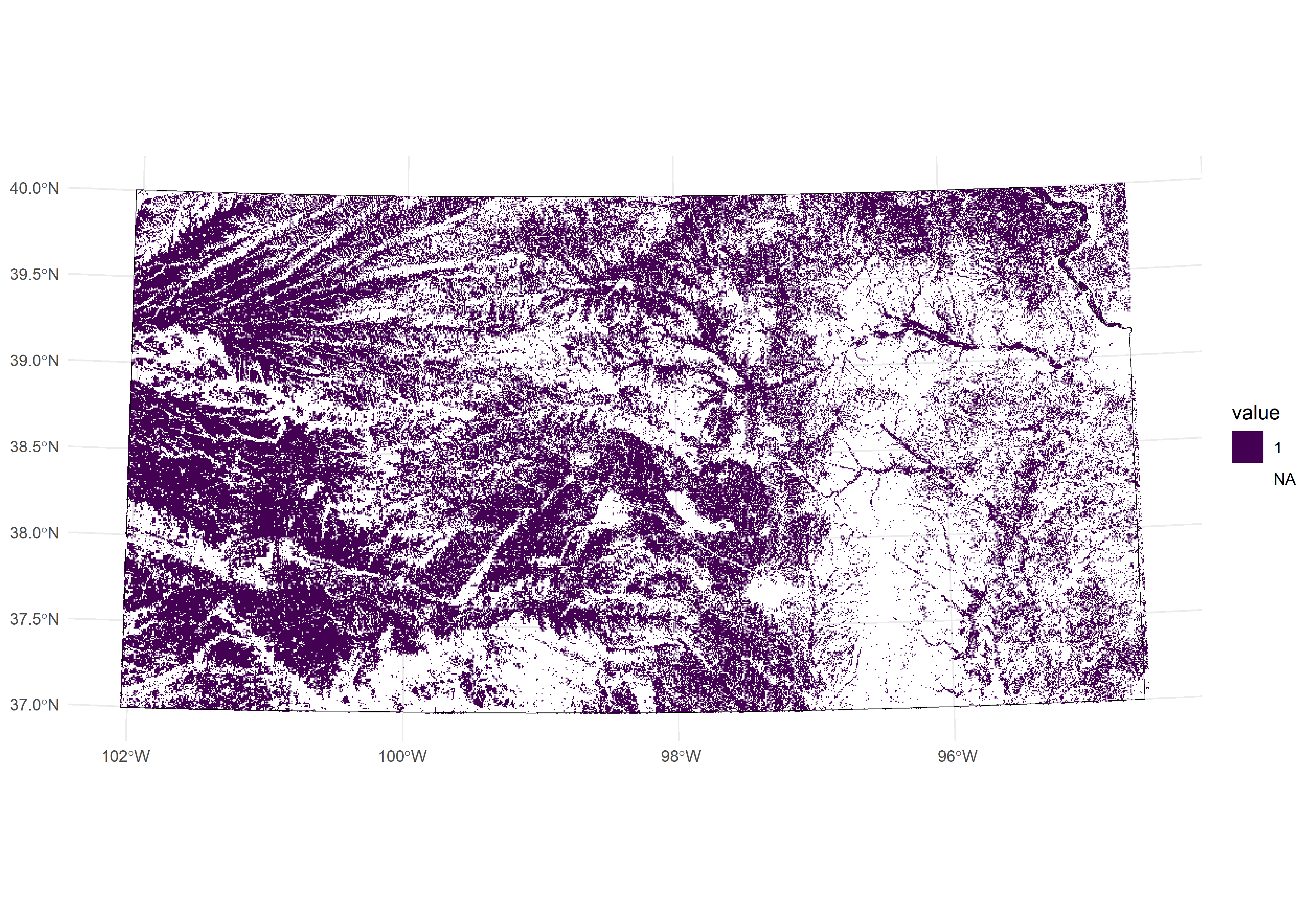
Figure 2.15: Spatial distribution of crops represented at the original pixel resolution (i.e., 16-meter pixel resolution).

The raster is resampled to 20 m resolution, which determines the spatial precision of TSU placement. This resolution directly controls sampling accuracy. Nearest-neighbor resampling is used to maintain categorical integrity.

# Create 20 m template
lulc_size_template <- rast(ext(crops), resolution = 20, crs = crs(crops))

crops <- as.factor(crops)
crops <- resample(crops, lulc_size_template, method = "near")

Optional spatial masks are applied: (i) npa excludes protected or restricted areas and (ii) slope excludes unsuitable terrain. These masks refine the sampling universe to feasible agricultural locations, increasing the likelihood that soil surveyors will be able to access the selected sites.

if(exists("npa")){
  crops <- mask(crops, npa)
}

if(exists("slope")){
  slope <- resample(slope, crops, method="near")
  crops <- crops * slope
}

# rm(npa, slope)

Table 2.9: Metadata of the resampled cropland mask raster.

Property	Value
Class	SpatRaster
Dimensions (rows, cols, layers)	17152 × 33243 × 1
Resolution (x, y)	20.00027 × 19.99955
Extent (xmin, xmax, ymin, ymax)	228591.3, 893460.4, 4093884, 4436916
Coordinate Reference System	NAD27 / UTM zone 14N (EPSG:26714)
Value Range	1–1 (binary mask)

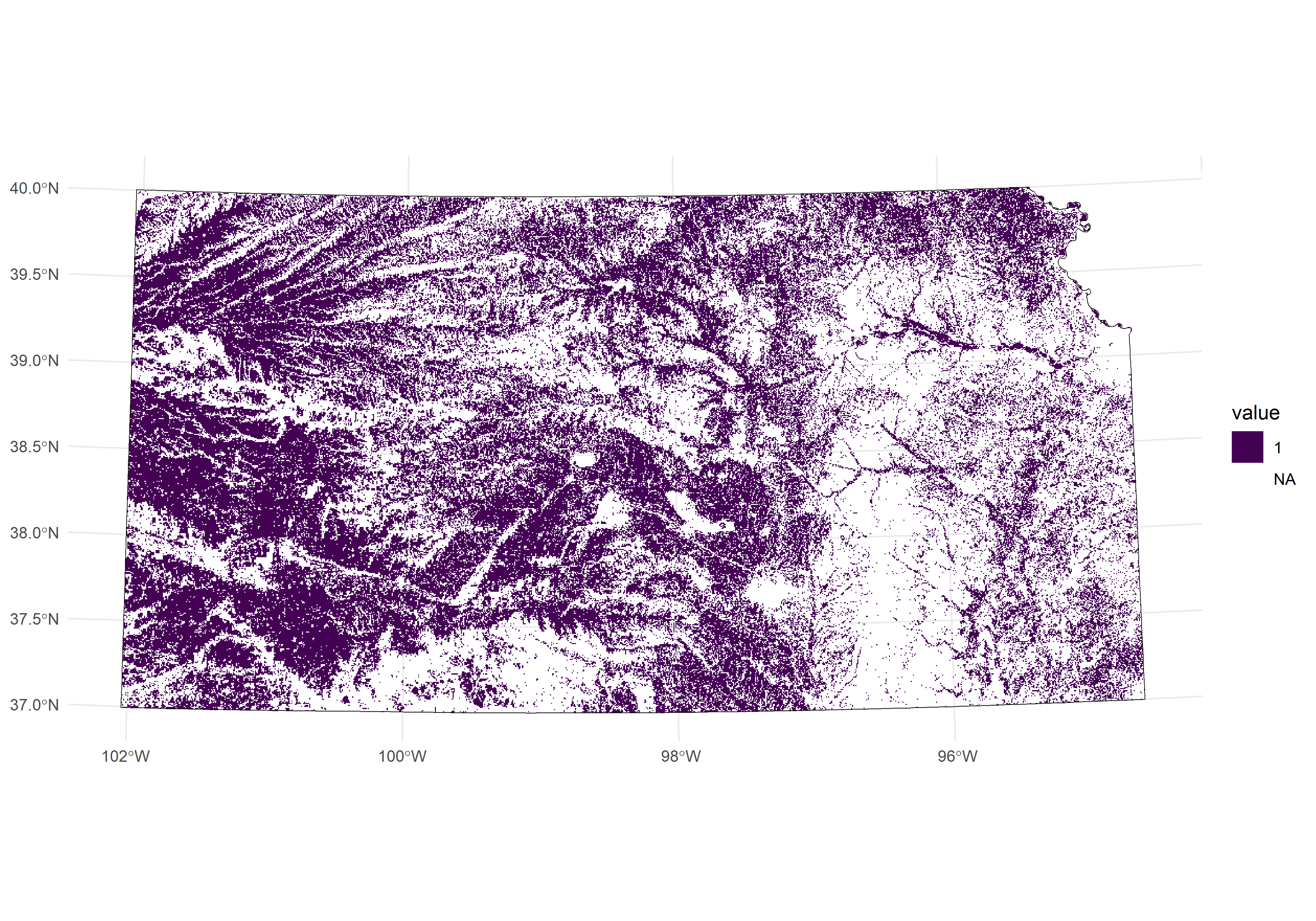
Figure 2.16: Spatial distribution of crops represented at 20-meter pixel resolution and excluding protected-areas and unaccessible slopes.

The processed 20 m cropland mask is saved and reloaded to ensure consistency and memory stability.

# Save 20m resolution crop mask
writeRaster(crops, paste0(raster.path,"crop_mask_20m_clean.tif"), overwrite=TRUE)
# Same situation as loading "cov.dat"
crops <- rast(paste0(raster.path,"crop_mask_20m_clean.tif"))

Aggregate to 100 m resolution

Resampling to 100 m resolution significantly optimises processing speed and reduces storage requirements. The 20 m raster is aggregated to 100 m resolution using the modal (majority) value. This coarser layer is used for PSU filtering and landscape-scale stratification at 1 ha (100 m x 100 m).

# Create 100m resolution version for PSU filtering
# Aggregate: (20m × 5) = 100m pixels
lu <- aggregate(crops, 5, fun=modal, cores = 4, na.rm=T)
names(lu) <- "lu"
writeRaster(lu, paste0(raster.path,"crop_mask_100m.tif"), overwrite=TRUE)
# Same situation as loading "cov.dat"
# lu <- rast(paste0(raster.path,"crop_mask_100m.tif"))

# Filter legacy data to crop areas
if (exists("legacy")){
  legacy$INSIDE <- terra::extract(crops, legacy) %>% dplyr::select(lu)
  legacy <- legacy[!is.na(legacy$INSIDE),] %>% dplyr::select(-"INSIDE")
}

# Display new resolution
lu

# Visualize (it takes a few minutes)
ggplot() +
  geom_spatraster(data = as.factor(crops)) +
  scale_fill_viridis_d(na.value = "transparent") +
  geom_spatvector(data = country_boundaries, fill = NA, color = "black") +
  geom_spatvector(data = legacy, size = 0.7, color = "red") +
  theme_minimal()

Table 2.10: Metadata of the resampled cropland mask raster at 100-metre pixel resolution.

Property	Value
Class	SpatRaster
Dimensions (rows, cols, layers)	3431 × 6649 × 1
Resolution (x, y)	100.0014 × 99.99777
Extent (xmin, xmax, ymin, ymax)	228591.3, 893500.4, 4093824, 4436916
Coordinate Reference System	NAD27 / UTM zone 14N (EPSG:26714)
Value Range	1–1 (binary mask)

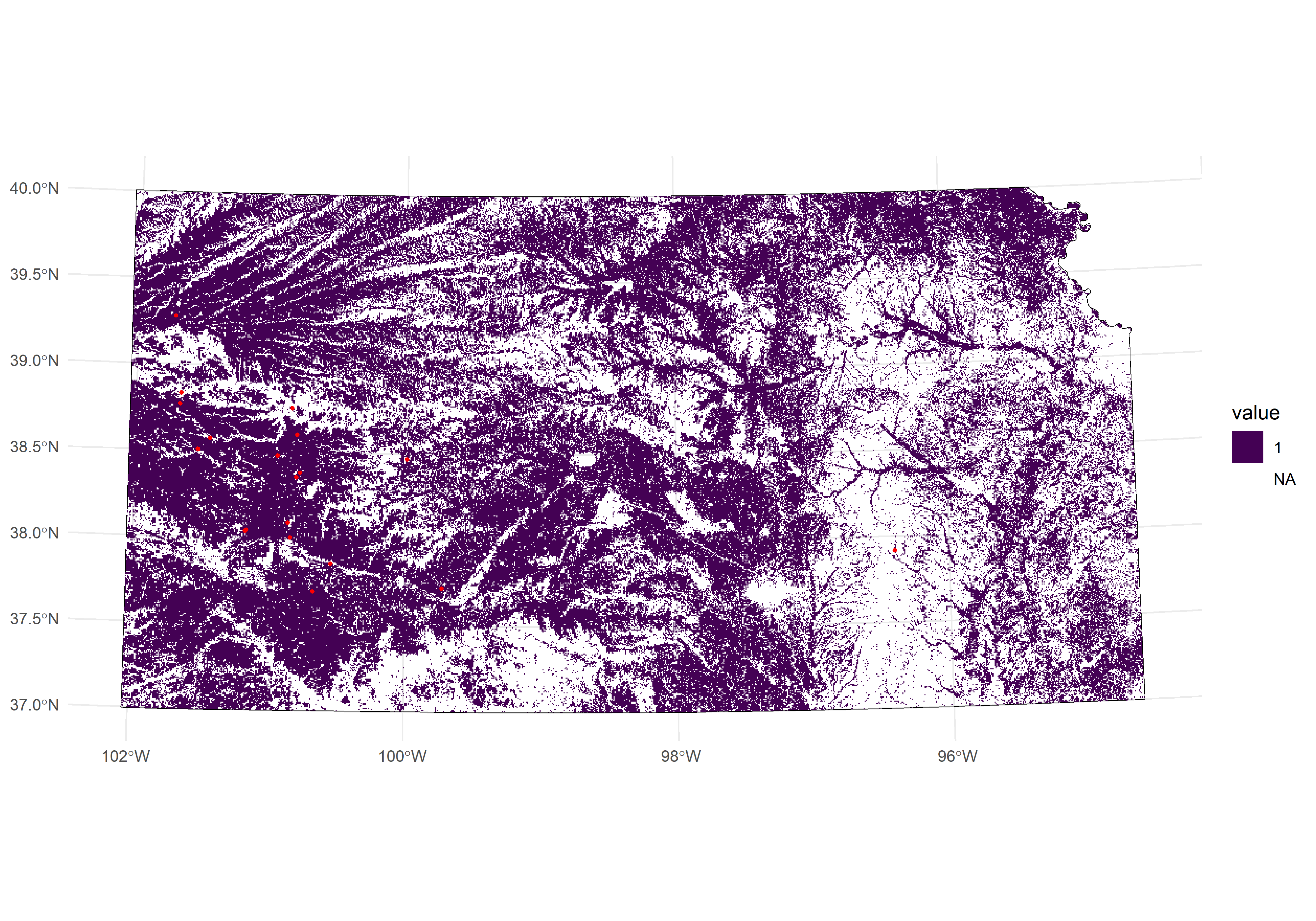
Figure 2.17: Spatial distribution of crops aggregated/upscaled from the original 20-meter pixel resolution to a coarser 100-meter pixel resolution for improved visualization and analysis.

2.4.9 Create Primary Sampling Units (PSU Grid)

A regular grid of PSUs was generated across the study area to establish a structured spatial sampling framework. PSUs represent fixed-area spatial units that serve as the primary level of sampling allocation and spatial stratification. A square grid with a resolution of 2 × 2 km was selected to balance spatial coverage and computational efficiency. This grid size ensures adequate representation of landscape variability, compatibility with aggregated environmental layers and operational feasibility for field-based sampling.

The grid was generated using the national boundary as a spatial reference and subsequently clipped to the study area to exclude regions outside the country limits. Each PSU was assigned a unique identifier to facilitate spatial indexing and downstream analyses. This PSU framework provides the foundation for hierarchical sampling, where finer-scale SSUs are nested within selected PSUs.

# Purpose: Create 2×2 km grid covering the study area

psu_grid <- st_make_grid(country_boundaries, cellsize = c(psu_size, psu_size), square = TRUE)
psu_grid <- st_sf(geometry = psu_grid)
psu_grid$ID <- 1:nrow(psu_grid)

# Clip to country boundary
psu_grid <- psu_grid[country_boundaries[1],]  # TIME CONSUMING!
write_sf(psu_grid, paste0(results.path,"../grid2k.shp"), overwrite=TRUE)

# Or load pre-saved grid (much faster)
# psu_grid <- sf::st_read(file.path(paste0(results.path,"../grid2k.shp")))

2.4.10 Select PSUs with sufficient land-use coverage

Not all 2 × 2 km PSUs contain enough cropland to justify sampling. This section quantifies cropland coverage within each PSU using the 100 m cropland mask and retains only those PSUs that exceed a minimum cropland threshold (e.g., 20%). Filtering PSUs in this way focuses sampling effort on agriculturally relevant areas and avoids allocating field effort to largely non-crop cells.

terra::extract() returns raster values per PSU polygon. Because lu is a binary cropland mask at 100 m resolution, summing lu within each PSU counts the number of 100 m cropland pixels. A 2 km PSU contains \((2000/100)^2 = 20^2 = 400\) pixels, so cropland percentage is computed as:

\[\% \text{cropland} = \frac{\sum lu}{400} \times 100\]

# Purpose: Keep only PSUs with sufficient cropland
# Why: No point sampling in PSUs with <20% crops

# Extract crop percentage for each PSU
extracted_values <- terra::extract(lu, psu_grid)

crop_perc <- extracted_values %>%
  group_by(ID) %>%
  summarize(crop_perc = sum(lu, na.rm = TRUE)*100/400)  # 400 = total of 100m pixels in 2km PSU

rm(extracted_values)

# Join back to PSU grid
psu_grid$crop_perc <- crop_perc$crop_perc
write_sf(psu_grid, file.path(paste0(results.path,"/psu_grid_counts.shp")), overwrite=TRUE)

# Reload and ensure correct projection (if R crashes!)
## Same as cov.dat and land use data
# psu_grid <- sf::st_read(file.path(paste0(results.path,"/psu_grid_counts.shp")))
# if(crs(psu_grid)!=epsg){
#   psu_grid <- psu_grid %>% sf::st_transform(crs=epsg)
# }

Visualize cropland coverage

# Visualize crop coverage
ggplot() +
  geom_sf(data = psu_grid, aes(fill = crop_perc)) +
  scale_fill_distiller(palette = "Spectral") +
  labs(title = "Crop Coverage by PSU", fill = "% Cropland") +
  theme_minimal()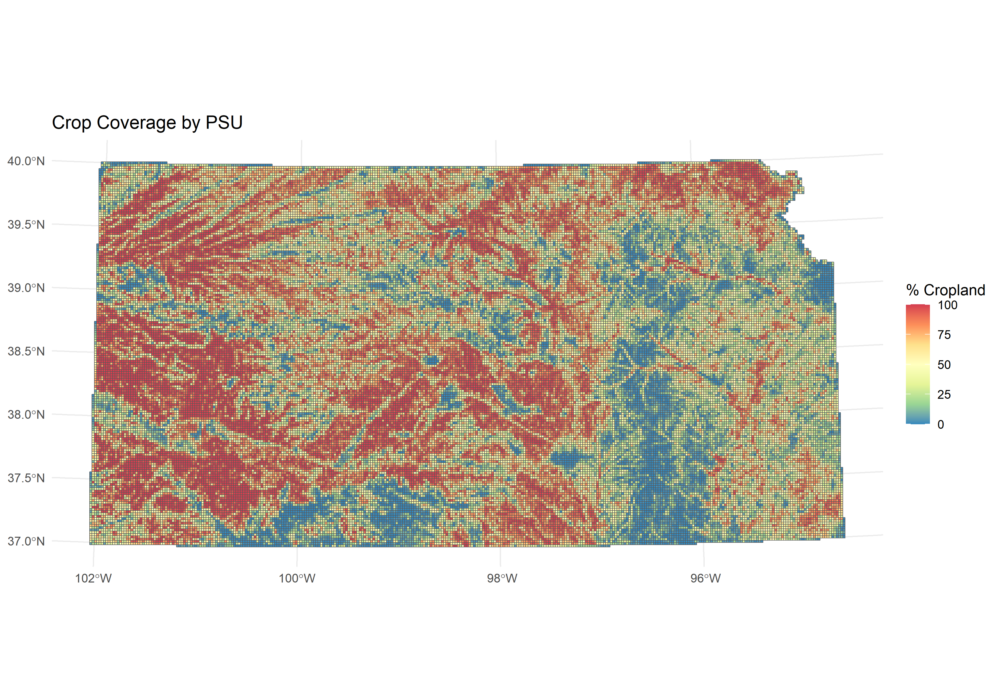

Figure 2.18: Percentage of cropland within each 2 x 2 km primary sampling unit (PSU), calculated from the 100 m cropland mask.

Filter PSUs based on cropland threshold

Only PSUs exceeding the minimum cropland threshold (percent_crop) are retained for subsequent TSU placement and sampling. This ensures that sampling effort is concentrated in PSUs where cropland is sufficiently prevalent to meet study objectives.

psu_grid <- psu_grid[psu_grid$crop_perc > percent_crop, "ID"]

cat(sprintf("Retained %d PSUs with > %d%% crop coverage\n", 
            nrow(psu_grid), percent_crop))

Rasterize PSUs for Covariate Space Coverage

The vector-based PSU grid is converted into raster format to enable efficient extraction and aggregation of environmental covariates. Rasterizing PSUs ensures spatial alignment with environmental covariates and allows cell-based operations for subsequent analysis (e.g., facilitating accurate clustering).

# Purpose: Convert vector PSUs to raster format for covariate extraction

template <- rast(vect(psu_grid), res = psu_size)
template <- rasterize(vect(psu_grid), template, field = "ID")

# Crop covariates to eligible PSUs only
cov.dat <- crop(cov.dat, psu_grid, mask=TRUE)
PSU.r <- resample(cov.dat, template)

2.4.11 Calculate optimal sample size

After rasterizing the PSUs for covariate space coverage, the optimal sample size is determined based on divergence metrics (Saurette et al., 2023). This section determines the optimal number of PSUs required to adequately represent environmental variability across the study area. Rather than selecting a sample size arbitrarily, a data-driven optimisation approach is applied to identify the point at which increasing the number of PSUs yields diminishing returns in environmental coverage.

# Purpose: Determine how many PSUs needed for representative coverage
# What this does:
#  - Tests different sample sizes (50, 75, 100, ... up to 3000 PSUs)
#  - Measures how well each sample size represents environmental variability
#  - Identifies the "sweet spot" where adding more PSUs gives diminishing returns
#  - Uses Kullback-Leibler divergence to compare sample vs population distributions
#
# Method: Feature Space Coverage (FCS) algorithm
#  - Iteratively samples PSUs and compares to full covariate space
#  - Repeats 4 times per sample size to ensure stability
#  - Selects optimal N where coverage reaches 95% of maximum
#
# COMPUTATION TIME: 
#  - Small areas (<1000 PSUs): 2-6 hours
#  - Medium areas (1000-5000 PSUs): 6-24 hours  
#  - Large areas (>5000 PSUs): 1-3 days
#  - Depends on: # of PSUs, # of covariates, CPU cores available
#
# SKIP THIS SECTION IF:
#  - You already ran it and saved the result (optimal_N_KLD.RDS exists)
#  - You have a predetermined sample size (e.g., budget constraints)
#  - Running quick tests (use arbitrary N like 50-100 PSUs)
#

source("scripts/opt_sample.R")  # Load optimization functions

psu.r.df <- data.frame(PSU.r)

# Optimization parameters
initial.n <- 50
final.n <- 3000
by.n <- 25
iters <- 4

# Run optimization (can take several minutes)
opt_N_fcs <- opt_sample(alg="fcs",
                        s_min=initial.n,
                        s_max=final.n,
                        s_step=by.n,
                        s_reps=iters,
                        covs = psu.r.df,
                        cpus=4,
                        conf=0.95)

optimal_N_KLD <- opt_N_fcs$optimal_sites[1,2]
cat(sprintf("Optimal sample size: %d PSUs\n", optimal_N_KLD))

saveRDS(optimal_N_KLD, paste0(results.path,"../optimal_N_KLD.RDS"))

💡 Note: The optimal sample size is based on Kullback-Leibler Divergence, which does not overestimate like Jensen-Shannon methods.

2.4.12 Select PSUs using Covariate Space Coverage (CSC)

After determining the target number of PSUs, the next step is to select PSU locations that maximise environmental diversity across the study area. The goal is not random spatial coverage, but coverage of the multivariate covariate space so that sampled PSUs collectively represent the dominant environmental gradients captured by the covariates (i.e., PCA components).

This section implements a CSC strategy using clustering in standardised covariate space. Selected PSUs correspond to cluster representatives and are interpreted as locations that best capture distinct portions of the environmental feature space. Sampling effort is allocated according to land-use priorities. In this example, the majority of PSUs are assigned to cropland. A buffer can be included to maintain the final target after excluding PSUs that fail feasibility checks later in the workflow.

# You can use the file from the repository for this exercise. 
optimal_N_KLD <- readRDS(paste0(results.path,"../optimal_N_KLD.RDS"))

# Proportional allocation by land-use class (adjust to study objectives)
crop_prop   <- 0.85
grass_prop  <- 0.10
forest_prop <- 0.05

# Number of PSUs allocated to cropland
n.psu <- round(optimal_N_KLD * crop_prop, 0)

# Optional buffer to account for exclusions during later steps
n.psu <- round(optimal_N_KLD * crop_prop * 1.15, 0)

cat(sprintf("Targeting %d PSUs for %s\n", n.psu, landuse)) # 412

Prepare PSU-level

Clustering is performed in standardised covariate space to ensure that each covariate contributes comparably. The resulting matrix (mygrd) represents each PSU as a point in multivariate feature space.

PSU.df <- as.data.frame(PSU.r, xy=T)
covs <- names(cov.dat)
mygrd <- data.frame(scale(PSU.df[, covs]))

Constrained clustering to respect legacy samples

If legacy sampling locations are available, they are incorporated using constrained clustering so that previously sampled PSUs remain part of the final design. Legacy points are matched to their nearest PSU representation and treated as fixed elements in the clustering solution. If no legacy data exists, standard k-means clustering is used to partition covariate space into n clusters.

# If legacy data exists, use constrained clustering
if (exists("legacy")){
  legacy <- st_filter(legacy, psu_grid)
  legacy_df <- st_coordinates(legacy)
  
  # Find nearest PSU for each legacy point
  units <- numeric(nrow(legacy_df))
  for (i in 1:nrow(legacy_df)) {
    distances <- sqrt((PSU.df$x - legacy_df[i, "X"])^2 + (PSU.df$y - legacy_df[i, "Y"])^2)
    units[i] <- which.min(distances)
  }
  
  fixed <- unique(data.frame(units, scale(PSU.df[, covs])[units, ]))
  
  # Run constrained clustering
  res <- CSIS(fixed = fixed, nsup = n.psu, nstarts = iterations, mygrd = mygrd)
  
} else {
  # No legacy data: standard k-means
  res <- kmeans_with_progress(mygrd, centers = n.psu, iter.max = 10000, nstart = iterations)
}

💡 Note: Progress is printed as “X out of Y” for each clustering iteration.

Select representative PSUs from cluster centers

Cluster centers exist in covariate space, not geographic space. Therefore, for each cluster center, the PSU with the minimum Euclidean distance in standardized covariate space is selected. These PSUs form the CSC sample because they are the closest realizations of the cluster “typical” environmental conditions.

# Assign cluster IDs
PSU.df$cluster <- res$cluster

# Find PSU closest to each cluster center (these become sample locations)
D <- rdist(x1 = res$centers, x2 = scale(PSU.df[, covs]))
units <- apply(D, MARGIN = 1, FUN = which.min)

myCSCsample <- PSU.df[units, c("x", "y", covs)]

Label legacy vs new selections and convert to spatial format

Selections are labeled to distinguish previously sampled PSUs (“legacy”) from newly proposed PSUs (“new”). The selected PSU representatives are then converted into an sf point layer for spatial overlay and mapping.

# Label legacy vs new PSUs
if (exists("legacy")){
  myCSCsample$type <- c(rep("legacy", nrow(fixed)), rep("new", length(units)-nrow(fixed)))
} else {
  myCSCsample$type <- "new"
}

# Convert to spatial object
myCSCsample <- myCSCsample %>%
  st_as_sf(coords = c("x", "y"), crs = epsg)

# Separate legacy and new
if (exists("legacy")){
  legacy <- myCSCsample[myCSCsample$type=="legacy",]
}
new <- myCSCsample[myCSCsample$type=="new",]

Identify target PSU polygons

Selected PSU representative points are intersected with the PSU polygon grid to recover the corresponding PSU IDs. The resulting polygon layer (target.PSUs) defines the final set of target PSUs for subsequent TSU placement.

# Extract target PSU IDs
PSUs <- sf::st_intersection(psu_grid, new) %>% dplyr::select(ID)
target.PSUs <- psu_grid[psu_grid$ID %in% PSUs$ID,] %>% dplyr::select(ID)

cat(sprintf("Selected %d target PSUs\n", nrow(target.PSUs)))

Output: The procedure returns n target PSUs, where n corresponds to the allocated sample size determined in the optimization step. These PSUs represent environmentally diverse sampling locations that collectively achieve the desired level of feature space coverage.

Visualise final outputs

ggplot() +
  geom_raster(data = as.data.frame(PSU.r$PC1, xy = TRUE), aes(x = x, y = y, fill = PC1)) +
  scale_fill_viridis_c() +
  geom_sf(data = target.PSUs, color = "#101010", fill = NA, lwd = 0.8) +
  geom_sf(data = new[1], color = "#D81B60", size = 0.5, shape = 19) +
  labs(title = "Target Primary Sampling Units") +
  theme_minimal()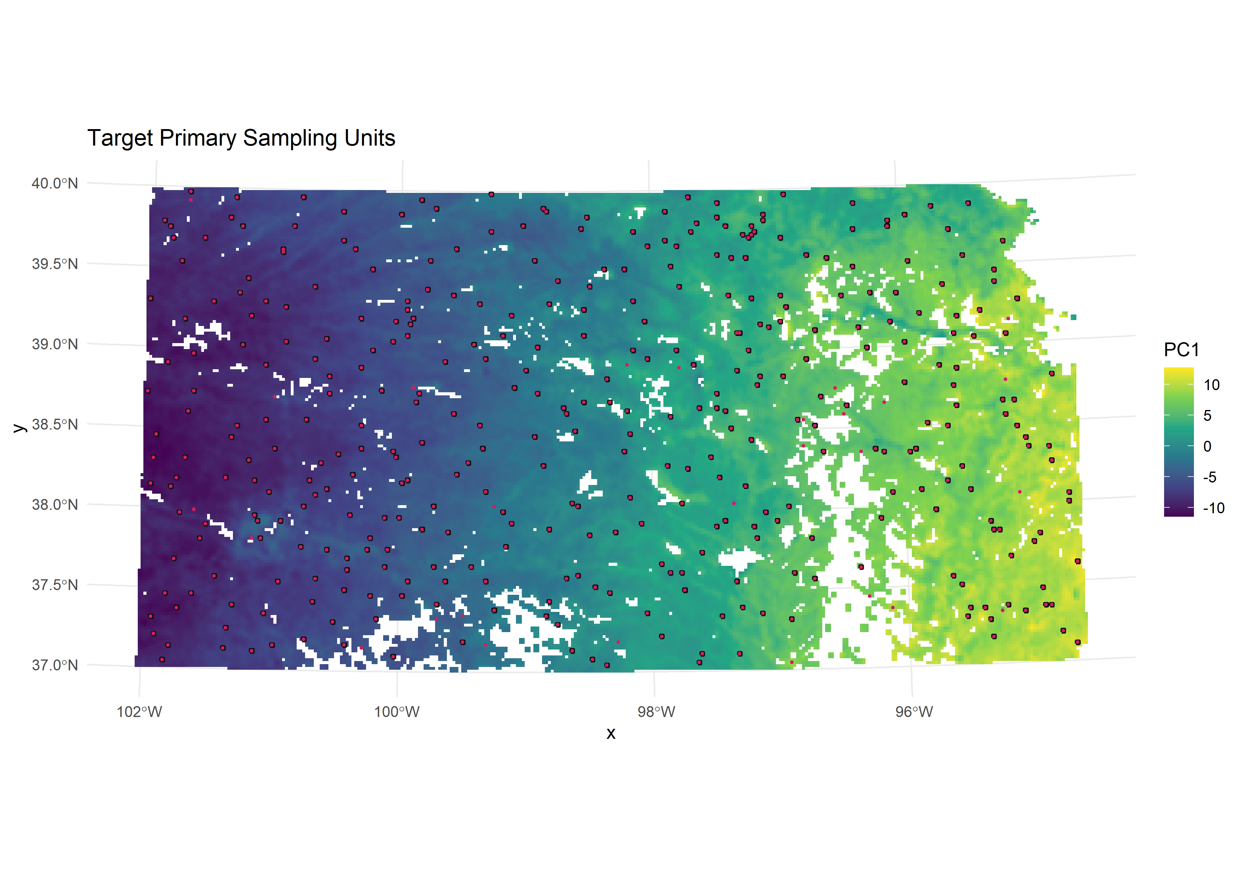

Figure 2.19: Distribution of selected target Primary Sampling Units over the covariate space coverage.

2.4.13 Compute SSUs and TSUs

Now we generate Secondary Sampling Units (100m × 100m) within each PSU and Tertiary Sampling Units (20m × 20m points) within each SSU.

Load high-resolution covariates

This section loads the high-resolution covariate raster stack (100 m) used to guide Secondary Sampling Unit (SSU) selection within each selected PSU. These covariates are distinct from the PSU-level covariates used earlier for PSU selection. At this stage, the objective is to capture within-PSU heterogeneity and support clustering or stratification at the SSU scale.

# Purpose: Load 100m resolution data for SSU clustering WITHIN each PSU
# Note: Different from PSU covariates - these determine SSU placement

cov.dat.ssu <- terra::rast(paste0(raster.path, "HighRes_Covariates_100m_KANSAS_merged.tif"))
names(cov.dat.ssu) <- gsub("(^\\d+_?S2_|^\\d+_|^S2_)", "", names(cov.dat.ssu))

if(crs(cov.dat.ssu)!=epsg){
  cov.dat.ssu <- terra::project(cov.dat.ssu, epsg, method="near")
}

# Check for and replace NA values
# Why: NA values cause complete.cases() to remove SSUs unnecessarily
# Solution: Replace NA with 0 (assumes missing data = no feature present)
if (any(is.na(values(cov.dat.ssu)))) {
  cat("Found NA values in SSU covariates. Replacing with 0...\n")
  na_count <- sum(is.na(values(cov.dat.ssu)))
  total_count <- ncell(cov.dat.ssu) * nlyr(cov.dat.ssu)
  cat(sprintf("Replacing %d NA values (%.2f%% of data)\n", 
              na_count, (na_count/total_count)*100))
  
  cov.dat.ssu[is.na(cov.dat.ssu)] <- 0
  
  cat("NA values replaced with 0\n\n")
} else {
  cat("No NA values found in SSU covariates\n\n")
}

writeRaster(cov.dat.ssu, paste0(raster.path,"cov_dat_ssu_100m_clean.tif"), overwrite=TRUE)
# Load if needed. Similar process to cov.dat and land use vars.
# cov.dat.ssu <- rast(paste0(raster.path,"cov_dat_ssu_100m_clean.tif"))

ssu_vars <- data.frame(
  Category = c(
    rep("Topography", 5),
    rep("Sentinel-2 Spectral Bands", 10),
    rep("Spectral Indices", 7)
  ),
  Variable = c(
    "SRTM_DEM", "Slope", "Aspect", "TPI", "Hillshade",
    "B2_Blue", "B3_Green", "B4_Red", "B5_RedEdge1", "B6_RedEdge2",
    "B7_RedEdge3", "B8_NIR", "B8A_NarrowNIR", "B11_SWIR1", "B12_SWIR2",
    "NDVI", "EVI", "NDBSI", "Redness_Index", "Brightness_Index",
    "NBRplus", "VNSIR"
  ),
  Description = c(
    "Digital Elevation Model (SRTM)",
    "Terrain slope derived from DEM",
    "Terrain aspect (orientation)",
    "Topographic Position Index",
    "Hillshade derived from DEM",
    "Blue band (490 nm)",
    "Green band (560 nm)",
    "Red band (665 nm)",
    "Red-edge band 1 (705 nm)",
    "Red-edge band 2 (740 nm)",
    "Red-edge band 3 (783 nm)",
    "Near-Infrared band (842 nm)",
    "Narrow Near-Infrared band (865 nm)",
    "Shortwave Infrared 1 (1610 nm)",
    "Shortwave Infrared 2 (2190 nm)",
    "Normalized Difference Vegetation Index",
    "Enhanced Vegetation Index",
    "Normalized Difference Bare Soil Index",
    "Redness spectral index",
    "Brightness index (composite reflectance)",
    "Normalized Burn Ratio (extended form)",
    "Visible and near-infrared spectral index"
  )
)

kable(ssu_vars,
      caption = "High-resolution (100 m) covariates used for SSU-level clustering.")

Core process of generating SSUs and TSUs

This section implements the core step of the three-stage sampling design. For each selected PSU, a grid of SSUs is generated and filtered to retain agriculturally valid units. SSU-level environmental covariates are then used to cluster SSUs and select a fixed number of target and replacement SSUs that represent within-PSU variability. Finally, TSU point locations are generated within each selected SSU, constrained to cropland pixels.

For each PSU in target.PSUs, the workflow proceeds as follows:

• Create SSU grid at 100 m resolution and clip it to the PSU boundary.

• Quantify cropland availability per SSU using the 20 m cropland mask and remove SSUs with insufficient valid crop pixels.

• Extract SSU-level covariates (100 m covariate stack) and prepare a standardized feature matrix for clustering.

• Cluster SSUs (k-means) to represent within-PSU environmental variation and select:

  • one SSU closest to each cluster center (Target SSUs), and

  • the second closest SSU (Replacement SSUs).

• Generate TSU points inside each target and replacement SSU, restricted to cropland cells.

Quality control: PSUs that fail any criterion (e.g., too few SSUs, covariate mismatches, incomplete cases, TSU generation failure) are skipped and recorded.

# Purpose: Within each target PSU, create SSUs and TSUs
# This is the CORE of the three-stage sampling design

# Initialize storage
all_psus_tsus <- list()
selected_ssus <- list()
skipped_psus <- c()

# MAIN LOOP: Process each target PSU
# MAIN LOOP: Process each target PSU to generate SSUs and TSUs
for (psu_id in 1:nrow(target.PSUs)) {
  
  # Select current PSU
  selected_psu <- target.PSUs[psu_id, ]
  
  # STEP 1: Generate 100m×100m SSU grid within the PSU boundary
  ssu_grid <- st_make_grid(selected_psu, cellsize = c(ssu_size, ssu_size), square = TRUE)
  ssu_grid_sf <- st_sf(geometry = ssu_grid)
  
  # Clip SSU grid to exact PSU boundary (removes partial cells outside PSU)
  ssu_grid_sf <- suppressWarnings(st_intersection(ssu_grid_sf, st_geometry(selected_psu)))
  
  # Convert to terra vector format for raster extraction
  ssu_grid_vect <- vect(ssu_grid_sf)
  
  # STEP 2: Calculate crop percentage for each SSU
  # Extracts from 20m resolution crop raster and calculates % coverage
  extracted_values <- extract(crops, ssu_grid_vect, fun = function(x) {
    sum(x > 0, na.rm = TRUE) / length(x) * 100
  })
  
  # Debug output: show range of crop coverage in this PSU
  cat(sprintf("\nPSU %d \n lu values range: %.2f to %.2f\n", 
              psu_id, min(extracted_values[,2]), max(extracted_values[,2])))
  
  # STEP 3: Verify extraction succeeded and assign crop values
  if (ncol(extracted_values) >= 2) {
    ssu_grid_sf$lu <- extracted_values[, 2]
    
    # STEP 4: Handle split geometries from st_intersection
    # st_intersection sometimes creates MULTIPOLYGON - we need to merge them back
    ssu_grid_sf$ssu_temp_id <- 1:nrow(ssu_grid_sf)  # Track original SSU IDs
    ssu_grid_sf <- st_cast(ssu_grid_sf, "POLYGON")  # Split any MULTIPOLYGONs
    
    # Merge split parts back to single polygons per SSU
    ssu_grid_sf <- ssu_grid_sf %>%
      group_by(ssu_temp_id, lu) %>%
      summarise(geometry = st_union(geometry), .groups = "drop") %>%
      select(-ssu_temp_id)  # Remove temporary ID
    
    # Store count before filtering for reporting
    total_ssus_before <- nrow(ssu_grid_sf)
    
    # STEP 5: Filter SSUs by actual 20m crop pixel count
    # This is more accurate than percentage and prevents TSU generation failures
    cat("Checking crop pixel availability for TSU generation...\n")
    ssu_grid_sf$crop_pixel_count <- sapply(1:nrow(ssu_grid_sf), function(i) {
      ssu_geom <- ssu_grid_sf[i, ]
      ssu_vect <- vect(ssu_geom)
      
      # Crop the 20m raster to this SSU and count valid pixels
      ssu_crop <- try(crop(crops, ssu_vect, mask = TRUE), silent = TRUE)
      if (inherits(ssu_crop, "try-error") || is.null(ssu_crop)) return(0)
      
      crop_vals <- values(ssu_crop, mat = FALSE)
      sum(crop_vals > 0, na.rm = TRUE)
    })
    
    # Minimum pixels needed: number of TSUs + safety buffer
    min_crop_pixels <- number_TSUs + 5
    ssu_grid_sf <- ssu_grid_sf[ssu_grid_sf$crop_pixel_count >= min_crop_pixels, ]
    
    # Report how many SSUs were removed
    cat(sprintf("SSUs after crop pixel filter: %d (removed %d)\n",
                nrow(ssu_grid_sf), total_ssus_before - nrow(ssu_grid_sf)))
    
  } else {
    # Extraction failed - skip this PSU
    warning(paste("PSU", psu_id, "returned insufficient extracted values. Skipping."))
    skipped_psus <- c(skipped_psus, psu_id)
    next
  }
  
  # Progress indicator
  cat(sprintf("\rProgress: %.2f%% (%d out of %d)\n", 
              (psu_id / nrow(target.PSUs)) * 100, psu_id, nrow(target.PSUs)))
  flush.console()
  
  # STEP 6: Check if enough SSUs remain for clustering
  total_ssus <- nrow(ssu_grid_sf)
  min_required_ssus <- max(num_primary_ssus + num_alternative_ssus, 8)  # Default: 4+4=8
  
  if (total_ssus < min_required_ssus) {
    warning(paste("PSU", psu_id, "has only", total_ssus, 
                  "usable SSUs (min required:", min_required_ssus, "). Skipping."))
    skipped_psus <- c(skipped_psus, psu_id)
    next
  }
  
  # STEP 7: Extract 100m environmental covariates for each SSU
  ssu_grid_vect_filtered <- vect(ssu_grid_sf)
  ssu_covariates <- terra::extract(cov.dat.ssu, ssu_grid_vect_filtered, df = TRUE)
  
  # Aggregate covariates if any SSUs were split (collapse to one row per SSU)
  ssu_covariates <- ssu_covariates %>%
    group_by(ID) %>%
    summarise(across(everything(), ~mean(.x, na.rm = TRUE)))
  
  # Verify SSU count matches covariate count (critical for alignment)
  if (nrow(ssu_covariates) != nrow(ssu_grid_sf)) {
    warning(sprintf("PSU %d: Mismatch in SSU and covariate rows (%d vs %d). Skipping.", 
                    psu_id, nrow(ssu_grid_sf), nrow(ssu_covariates)))
    skipped_psus <- c(skipped_psus, psu_id)
    next
  }
  
  # STEP 8: Prepare covariates for k-means clustering
  # Combine spatial data with environmental covariates
  ssu_data <- cbind(ssu_grid_sf, ssu_covariates[, -1])
  ssu_data_values <- st_drop_geometry(ssu_data)
  
  # Separate categorical variables (don't scale these)
  exclude <- grep("^geomorph_|^lu$", names(ssu_data_values), value = TRUE)
  to_scale <- ssu_data_values[, !names(ssu_data_values) %in% exclude]
  to_keep  <- ssu_data_values[, names(ssu_data_values) %in% exclude, drop = FALSE]
  
  # Remove columns with all NA values
  to_scale <- to_scale[, colSums(!is.na(to_scale)) > 0, drop = FALSE]
  
  # Identify zero-variance columns (would cause scaling errors)
  zero_variance_cols <- sapply(to_scale, function(x) sd(x, na.rm = TRUE) == 0)
  zero_variance_cols[is.na(zero_variance_cols)] <- TRUE
  
  # Scale only non-zero-variance columns
  scaled_part <- to_scale
  if (any(!zero_variance_cols)) {
    scaled_part[, !zero_variance_cols] <- scale(to_scale[, !zero_variance_cols])
  }
  
  # STEP 9: Remove incomplete cases and keep ssu_data aligned
  mygrd_ssu <- cbind(to_keep, scaled_part)
  complete_rows <- complete.cases(mygrd_ssu)
  mygrd_ssu <- mygrd_ssu[complete_rows, ]
  ssu_data <- ssu_data[complete_rows, ]  # CRITICAL: Keep aligned with mygrd_ssu!
  
  # Verify enough SSUs remain after removing incomplete cases
  if (nrow(mygrd_ssu) < 4) {
    warning(paste("PSU", psu_id, "has too few SSUs (", nrow(mygrd_ssu), ") to form 4 clusters. Skipping."))
    skipped_psus <- c(skipped_psus, psu_id)
    next
  }
  
  # STEP 10: Cluster SSUs using k-means
  # Number of clusters = number of target SSUs needed
  optimal_k <- num_primary_ssus
  
  kmeans_result <- kmeans(mygrd_ssu[, -1, drop = FALSE], centers = optimal_k, iter.max = 10000, nstart = 10)
  ssu_data$cluster <- as.factor(kmeans_result$cluster)
  
  # STEP 11: Select SSUs closest to cluster centers
  # These become target and replacement SSUs
  D <- rdist(x1 = kmeans_result$centers, x2 = mygrd_ssu[, -1, drop = FALSE])
  target_units <- apply(D, 1, function(x) order(x)[1])      # 1st closest = target
  replacement_units <- apply(D, 1, function(x) order(x)[2]) # 2nd closest = replacement
  
  # Verify we got enough SSUs
  if (length(target_units) < num_primary_ssus || length(replacement_units) < num_alternative_ssus) {
    warning(sprintf("PSU %d did not yield", num_primary_ssus ,"target and", num_alternative_ssus, "replacement SSUs. Skipping.", psu_id))
    skipped_psus <- c(skipped_psus, psu_id)
    next
  }
  
  # STEP 12: Extract selected SSUs and add metadata
  target_ssus <- ssu_data[target_units, ]
  replacement_ssus <- ssu_data[replacement_units, ]
  
  target_ssus$SSU_Type <- "Target"
  replacement_ssus$SSU_Type <- "Replacement"
  target_ssus$SSU_ID <- 1:nrow(target_ssus)
  replacement_ssus$SSU_ID <- (nrow(target_ssus) + 1):(2 * nrow(target_ssus))
  
  # Link each replacement SSU to its corresponding target SSU (same cluster)
  replacement_ssus$replacement_for <- sapply(replacement_ssus$cluster, function(cl) {
    matched <- target_ssus$SSU_ID[target_ssus$cluster == cl]
    if (length(matched) > 0) return(matched[1]) else return(NA)
  })
  
  target_ssus$replacement_for <- NA
  
  # Add PSU identifier
  psu_actual_id <- selected_psu$ID
  target_ssus$PSU_ID <- psu_actual_id
  replacement_ssus$PSU_ID <- psu_actual_id
  
  # Combine target and replacement SSUs
  combined_ssus <- rbind(target_ssus, replacement_ssus)
  
  # STEP 13: Final check - must have exactly expected number of SSUs
  if (nrow(combined_ssus) != (num_primary_ssus + num_alternative_ssus)) {
    warning(sprintf("PSU %d has %d SSUs instead of", num_primary_ssus + num_alternative_ssus, ". Skipping.", psu_id, nrow(combined_ssus)))
    skipped_psus <- c(skipped_psus, psu_id)
    next
  }
  
  # Store SSUs for this PSU
  selected_ssus[[psu_id]] <- combined_ssus
  
  # STEP 14: Generate TSU point samples within each SSU
  primary_tsus <- lapply(1:nrow(target_ssus), function(i) {
    generate_tsu_points_within_ssu(target_ssus[i, ], number_TSUs, target_ssus$SSU_ID[i], "Target", crops)
  })
  
  alternative_tsus <- lapply(1:nrow(replacement_ssus), function(i) {
    generate_tsu_points_within_ssu(replacement_ssus[i, ], number_TSUs, replacement_ssus$SSU_ID[i], "Replacement", crops)
  })
  
  # STEP 15: Verify all TSUs were generated successfully
  all_tsus <- c(primary_tsus, alternative_tsus)
  tsu_counts <- sapply(all_tsus, function(x) if(is.null(x)) 0 else nrow(x))
  
  # Check: each SSU must have exactly number_TSUs points
  if (any(tsu_counts != number_TSUs)) {
    warning(sprintf("PSU %d: TSU generation failed for some SSUs. Expected %d TSUs per SSU, got: %s. Skipping.", 
                    psu_id, number_TSUs, paste(tsu_counts, collapse=",")))
    skipped_psus <- c(skipped_psus, psu_id)
    # Remove this PSU from selected SSUs (failed at final step)
    selected_ssus[[psu_id]] <- NULL
    next
  }
  
  # Store all TSUs for this PSU
  all_psus_tsus[[psu_id]] <- do.call(rbind, Filter(Negate(is.null), all_tsus))
}

Processing Summary:
For each PSU, the loop reports:

• The range of cropland coverage across generated SSUs (lu values range).
• The number of SSUs remaining after enforcing the minimum crop pixel threshold.
• The number of SSUs removed due to insufficient cropland.
• A real-time progress indicator showing the percentage completed and the current PSU index.

Example:
For PSU 20, cropland coverage ranged from 0% to 100%. After applying the crop pixel filter, 278 SSUs remained and 122 SSUs were removed. At this point, the overall progress was 5.32% (20 out of 376 PSUs processed).

This detailed reporting ensures transparency of SSU filtering and allows monitoring of computational progress during execution.

# Summary
cat(sprintf("Successfully processed: %d PSUs\n", length(selected_ssus)))
cat(sprintf("Skipped: %d PSUs\n", length(skipped_psus)))
if (length(skipped_psus) > 0) {
  cat(sprintf("Skipped PSU IDs: %s\n", paste(skipped_psus, collapse = ", ")))
}

Combine and structure SSUs and TSUs

This section consolidates the TSU point samples generated across all processed PSUs into a single, well-structured spatial dataset. SSU metadata (e.g., target vs replacement status and replacement links) are joined to each TSU to support field implementation, traceability, and downstream reporting.

# Purpose: Merge all TSUs into single spatial dataset with proper structure

all_ssus <- do.call(rbind, selected_ssus)
all_ssus <- all_ssus %>% mutate_at(vars(PSU_ID, SSU_ID), as.numeric)

all_tsus <- do.call(rbind, all_psus_tsus)
all_tsus <- all_tsus %>% mutate_at(vars(PSU_ID, SSU_ID), as.numeric)

# Join TSU and SSU metadata
all_tsus <- st_join(all_tsus, all_ssus[c("PSU_ID", "SSU_ID", "SSU_Type", "replacement_for")])

all_tsus <- all_tsus %>%
  select(PSU_ID = PSU_ID.x, SSU_ID = SSU_ID.y, SSU_Type = SSU_Type.y,
         Replacement_for = replacement_for, TSU_ID, geometry)

# Label TSU types (Target = primary sample, Alternative = backup)
all_tsus <- all_tsus %>%
  group_by(PSU_ID) %>%
  filter(n() == (num_primary_ssus + num_alternative_ssus) * number_TSUs) %>%  # 24 for default
  group_by(PSU_ID, SSU_ID) %>%
  mutate(TSU_Type = ifelse(row_number() == 1, "Target", "Alternative")) %>%
  ungroup()

all_tsus$PSU_Type <- "Target"

all_tsus <- all_tsus %>%
  dplyr::select("PSU_ID", "SSU_ID", "SSU_Type", "Replacement_for", 
                "TSU_ID", "TSU_Type", "geometry")

# Count target samples
n_target_tsus <- all_tsus %>%
  filter(SSU_Type == "Target" & TSU_Type == "Target") %>%
  distinct(PSU_ID, SSU_ID) %>%
  nrow()

cat(sprintf("\nTotal target sampling locations: %d\n", n_target_tsus))

Output: The resulting dataset (all_tsus) is the finalised TSU sampling frame, where each point includes its PSU and SSU identifiers, SSU status (target vs replacement), and TSU status (target vs alternative). This structure supports both field navigation and reproducible linking of observations to the sampling design.

Visualise final outputs

ggplot() +
  geom_raster(data = as.data.frame(PSU.r$PC1, xy = TRUE), aes(x = x, y = y, fill = PC1)) +
  scale_fill_viridis_c() +
  geom_sf(data = target.PSUs, color = "#101010", fill = NA, lwd = 0.8) +
  geom_sf(data = new[1], color = "#D81B60", size = 0.5, shape = 19) +
  labs(title = "Target Primary Sampling Units") +
  theme_minimal()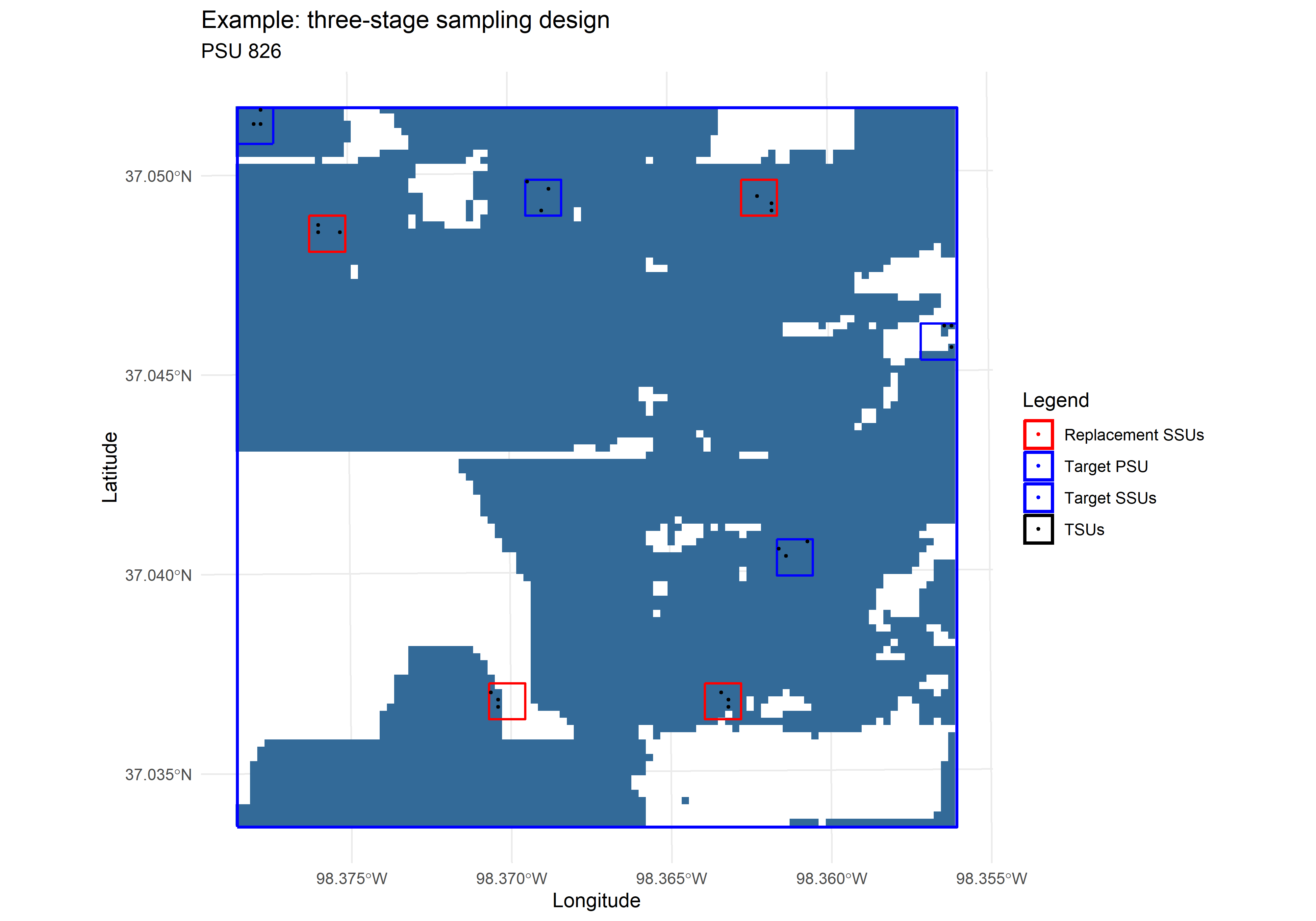

Figure 2.20: Illustration of the hierarchical three-stage sampling design showing the PSU boundary, selected SSUs (i.e., target and replacement), and TSU point locations within a representative PSU.

Export sampling units

This section prepares and exports the final spatial layers required for field implementation. Specifically, cluster information is attached to PSUs and TSUs, a consistent sampling order and unique site identifiers are generated, and the finalized PSU/TSU layers are written to disk as shapefiles plus a raster of clusters for reference.

# Purpose: Save all shapefiles for field work

# Add cluster information
dfr <- PSU.df[,c("x","y","cluster")]
dfr$cluster <- as.numeric(dfr$cluster)
dfr <- rasterFromXYZ(dfr)
crs(dfr) <- epsg

valid.PSU_clusters <- target.PSUs %>% 
  mutate(cluster = extract(dfr, target.PSUs, fun = mean, na.rm = TRUE))

all.PSU_clusters <- psu_grid %>% 
  mutate(cluster = extract(dfr, psu_grid, fun = mean, na.rm = TRUE))

all.PSU_clusters <- na.omit(all.PSU_clusters)

valid.PSU_clusters <- valid.PSU_clusters %>% rename(Replace_ID = cluster)

# Join cluster info to TSUs
all_tsus <- st_join(all_tsus, valid.PSU_clusters)

# Add sampling order
all_tsus <- all_tsus %>%
  group_by(PSU_ID) %>%
  mutate(order = match(SSU_ID, unique(SSU_ID))) %>%
  ungroup()

# Create unique site IDs
# Format: [COUNTRY CODE][PSU ID]-[SSU ID]-[TSU ID][LAND USE]
# Example: KANSAS0001-1-1C (PSU 1, SSU 1, TSU 1, Cropland)
all_tsus$site_id <- paste0(ISO.code, sprintf("%04d", all_tsus$PSU_ID), 
                           "-", all_tsus$SSU_ID, 
                           "-", all_tsus$TSU_ID, "C")  # C for Cropland

# Filter valid PSUs (those with complete TSU sets)
psus_with_tsus <- unique(all_tsus$PSU_ID)
valid.PSU_clusters_filtered <- valid.PSU_clusters %>%
  filter(ID %in% psus_with_tsus)

# Export shapefiles
write_sf(valid.PSU_clusters_filtered, 
         paste0(results.path,"/PSUs_target.shp"), overwrite=TRUE)
write_sf(all_tsus, 
         paste0(results.path,"/TSUs_target.shp"), overwrite=TRUE)
write_sf(all.PSU_clusters, 
         paste0(results.path,"/PSU_pattern_cl.shp"), overwrite=TRUE)
writeRaster(dfr, paste0(results.path,"/clusters.tif"), overwrite=TRUE)

2.4.14 Compute Alternative PSUs

Field sampling designs typically require contingency options because some target PSUs may become inaccessible (e.g., access restrictions, flooded roads, crop harvest, safety constraints). To maintain environmental representativeness while providing operational flexibility, a replacement PSU is selected for each target PSU cluster. Replacements are chosen from the same cluster as the target PSU, ensuring that the replacement PSU is environmentally similar in the multivariate covariate space.

Generate replacement PSUs from the same environmental clusters as targets.

# Purpose: For each target PSU, find a similar replacement in same cluster
# Why: Field teams need backups if target PSU becomes inaccessible

# Find PSUs NOT selected as targets
remaining.PSU_clusters <- all.PSU_clusters %>%
  filter(!(ID %in% valid.PSU_clusters$ID))

# Get unique cluster IDs from targets
unique_cluster <- distinct(valid.PSU_clusters, Replace_ID)$Replace_ID

# Sample one replacement per cluster
sampled_indices <- integer(0)

for (clust in unique_cluster) {
  candidates_indices <- which(remaining.PSU_clusters$cluster == clust)
  
  if (length(candidates_indices) > 0) {
    sampled_index <- sample(candidates_indices, size = 1)
    sampled_indices <- c(sampled_indices, sampled_index)
  }
}

replacements <- remaining.PSU_clusters[sampled_indices, ]

cat(sprintf("Selected %d replacement PSUs\n", nrow(replacements)))

Output: The object replacements contain one backup PSU per target cluster, where available. These replacement PSUs can be used by field teams if a target PSU cannot be sampled, while preserving the intended environmental coverage of the sampling design.

Generating SSUs and TSUs for replacement PSUs

Following the same procedure used for the target PSUs, SSUs and TSUs are generated within each replacement PSU. This ensures that backup PSUs are fully prepared for field deployment and maintain consistency with the three-stage sampling design. The process replicates SSU grid creation, covariate-based clustering, and TSU point generation, guaranteeing that replacement PSUs are operationally equivalent to their corresponding target PSUs.

# Purpose: Create same sampling structure in replacement PSUs
# Note: Code is identical to target PSU loop (Section 15)

alt_psus_tsus_sf <- list()
selected_ssus_sf <- list()
skipped_psus_sf <- c()

# DUPLICATE OF MAIN LOOP FOR REPLACEMENTS
# (See Section 15 for detailed comments)
for (psu_id in 1:nrow(replacements)) {
  selected_psu <- replacements[psu_id, ]
  
  # Generate SSUs within the selected PSU
  ssu_grid <- st_make_grid(selected_psu, cellsize = c(ssu_size, ssu_size), square = TRUE)
  ssu_grid_sf <- st_sf(geometry = ssu_grid)
  ssu_grid_sf <- suppressWarnings(st_intersection(ssu_grid_sf, st_geometry(selected_psu)))
  ssu_grid_vect <- vect(ssu_grid_sf)
  
  # Extract land use values (LU)
  extracted_values <- extract(crops, ssu_grid_vect, fun = function(x) {
    sum(x > 0, na.rm = TRUE) / length(x) * 100
  })
  
  # ADD THIS DEBUG LINE:
  cat(sprintf("\nPSU %d\n lu values range: %.2f to %.2f\n", 
              psu_id, min(extracted_values[,2]), max(extracted_values[,2])))
  
  # Defensive check: ensure extracted_values has at least 2 columns
  if (ncol(extracted_values) >= 2) {
    ssu_grid_sf$lu <- extracted_values[, 2]
    
    # FIX: Handle MULTIPOLYGON geometries that cause row mismatches
    ssu_grid_sf$ssu_temp_id <- 1:nrow(ssu_grid_sf)
    ssu_grid_sf <- st_cast(ssu_grid_sf, "POLYGON")
    
    # Group split geometries back together
    ssu_grid_sf <- ssu_grid_sf %>%
      group_by(ssu_temp_id, lu) %>%
      summarise(geometry = st_union(geometry), .groups = "drop") %>%
      select(-ssu_temp_id)
    
    # Store count before filtering
    total_ssus_before <- nrow(ssu_grid_sf)
    
    # ONLY USE THIS FILTER: Direct pixel count (accurate!)
    cat("Checking crop pixel availability for TSU generation...\n")
    ssu_grid_sf$crop_pixel_count <- sapply(1:nrow(ssu_grid_sf), function(i) {
      ssu_geom <- ssu_grid_sf[i, ]
      ssu_vect <- vect(ssu_geom)
      ssu_crop <- try(crop(crops, ssu_vect, mask = TRUE), silent = TRUE)
      if (inherits(ssu_crop, "try-error") || is.null(ssu_crop)) return(0)
      crop_vals <- values(ssu_crop, mat = FALSE)
      sum(crop_vals > 0, na.rm = TRUE)
    })
    
    min_crop_pixels <- number_TSUs + 5
    ssu_grid_sf <- ssu_grid_sf[ssu_grid_sf$crop_pixel_count >= min_crop_pixels, ]
    
    cat(sprintf("SSUs after crop pixel filter: %d (removed %d)\n",
                nrow(ssu_grid_sf), total_ssus_before - nrow(ssu_grid_sf)))
    
  } else {
    warning(paste("PSU", psu_id, "returned insufficient extracted values. Skipping."))
    skipped_psus_sf <- c(skipped_psus_sf, psu_id)
    next
  }
  
  cat(sprintf("\rProgress: %.2f%% (%d out of %d)\n", 
              (psu_id / nrow(replacements)) * 100, psu_id, nrow(replacements)))
  flush.console()
  
  # Count available SSUs
  total_ssus <- nrow(ssu_grid_sf)
  min_required_ssus <- max(num_primary_ssus + num_alternative_ssus, 8)  # 4 clusters x 2 SSUs each
  
  if (total_ssus < min_required_ssus) {
    warning(paste("PSU", psu_id, "has only", total_ssus, 
                  "usable SSUs (min required:", min_required_ssus, "). Skipping."))
    skipped_psus_sf <- c(skipped_psus_sf, psu_id)
    next
  }
  
  # Extract covariates
  # Convert filtered SSU grid to vector and extract covariates *after filtering*
  ssu_grid_vect_filtered <- vect(ssu_grid_sf)
  ssu_covariates <- terra::extract(cov.dat.ssu, ssu_grid_vect_filtered, df = TRUE)
  
  ssu_covariates <- ssu_covariates %>%
    group_by(ID) %>%
    summarise(across(everything(), ~mean(.x, na.rm = TRUE)))
  
  # Ensure alignment by checking row counts before binding
  if (nrow(ssu_covariates) != nrow(ssu_grid_sf)) {
    warning(sprintf("PSU %d: Mismatch in SSU and covariate rows (%d vs %d). Skipping.", 
                    psu_id, nrow(ssu_grid_sf), nrow(ssu_covariates)))
    skipped_psus_sf <- c(skipped_psus_sf, psu_id)
    next
  }
  
  ssu_data <- cbind(ssu_grid_sf, ssu_covariates[, -1])
  ssu_data_values <- st_drop_geometry(ssu_data)
  
  exclude <- grep("^geomorph_|^lu$", names(ssu_data_values), value = TRUE)
  to_scale <- ssu_data_values[, !names(ssu_data_values) %in% exclude]
  to_keep  <- ssu_data_values[, names(ssu_data_values) %in% exclude, drop = FALSE]
  
  to_scale <- to_scale[, colSums(!is.na(to_scale)) > 0, drop = FALSE]
  zero_variance_cols <- sapply(to_scale, function(x) sd(x, na.rm = TRUE) == 0)
  zero_variance_cols[is.na(zero_variance_cols)] <- TRUE
  
  scaled_part <- to_scale
  if (any(!zero_variance_cols)) {
    scaled_part[, !zero_variance_cols] <- scale(to_scale[, !zero_variance_cols])
  }
  
  mygrd_ssu <- cbind(to_keep, scaled_part)
  complete_rows <- complete.cases(mygrd_ssu)
  mygrd_ssu <- mygrd_ssu[complete_rows, ]
  # Also filter ssu_data to match
  ssu_data <- ssu_data[complete_rows, ]
  
  if (nrow(mygrd_ssu) < 4) {
    warning(paste("PSU", psu_id, "has too few SSUs (", nrow(mygrd_ssu), ") to form 4 clusters. Skipping."))
    skipped_psus_sf <- c(skipped_psus_sf, psu_id)
    next
  }
  
  # Fixed number of clusters
  optimal_k <- num_primary_ssus
  
  kmeans_result <- kmeans(mygrd_ssu[, -1, drop = FALSE], centers = optimal_k, iter.max = 10000, nstart = 10)
  ssu_data$cluster <- as.factor(kmeans_result$cluster)
  
  # Compute distances and pick SSUs closest to centers
  D <- rdist(x1 = kmeans_result$centers, x2 = mygrd_ssu[, -1, drop = FALSE])
  target_units <- apply(D, 1, function(x) order(x)[1])
  replacement_units <- apply(D, 1, function(x) order(x)[2])
  
  if (length(target_units) < num_primary_ssus || length(replacement_units) < num_alternative_ssus) {
    warning(sprintf("PSU %d did not yield", num_primary_ssus ,"target and", num_alternative_ssus, "replacement SSUs. Skipping.", psu_id))
    skipped_psus_sf <- c(skipped_psus_sf, psu_id)
    next
  }
  
  target_ssus <- ssu_data[target_units, ]
  replacement_ssus <- ssu_data[replacement_units, ]
  
  target_ssus$SSU_Type <- "Target"
  replacement_ssus$SSU_Type <- "Replacement"
  target_ssus$SSU_ID <- 1:nrow(target_ssus)
  replacement_ssus$SSU_ID <- (nrow(target_ssus) + 1):(2 * nrow(target_ssus))
  
  replacement_ssus$replacement_for <- sapply(replacement_ssus$cluster, function(cl) {
    matched <- target_ssus$SSU_ID[target_ssus$cluster == cl]
    if (length(matched) > 0) return(matched[1]) else return(NA)
  })
  
  target_ssus$replacement_for <- NA
  
  # Add PSU_ID and combine
  psu_actual_id <- selected_psu$ID
  target_ssus$PSU_ID <- psu_actual_id
  replacement_ssus$PSU_ID <- psu_actual_id
  # Combine SSUs
  combined_ssus <- rbind(target_ssus, replacement_ssus)
  
  # CHECK: Must have exactly 8 SSUs (4 target + 4 replacement)
  if (nrow(combined_ssus) != (num_primary_ssus + num_alternative_ssus)) {
    warning(sprintf("PSU %d has %d SSUs instead of", num_primary_ssus + num_alternative_ssus, ". Skipping.", psu_id, nrow(combined_ssus)))
    skipped_psus_sf <- c(skipped_psus_sf, psu_id)
    next
  }
  
  # Store only if we have exactly 8 SSUs
  selected_ssus_sf[[psu_id]] <- combined_ssus
  
  ### Generate TSUs ###
  primary_tsus <- lapply(1:nrow(target_ssus), function(i) {
    generate_tsu_points_within_ssu(target_ssus[i, ], number_TSUs, target_ssus$SSU_ID[i], "Target", crops)
  })
  
  alternative_tsus <- lapply(1:nrow(replacement_ssus), function(i) {
    generate_tsu_points_within_ssu(replacement_ssus[i, ], number_TSUs, replacement_ssus$SSU_ID[i], "Replacement", crops)
  })
  
  # CHECK: Verify all TSUs were generated successfully
  all_tsus <- c(primary_tsus, alternative_tsus)
  tsu_counts <- sapply(all_tsus, function(x) if(is.null(x)) 0 else nrow(x))
  
  # Each SSU should have exactly number_TSUs (3) TSUs
  if (any(tsu_counts != number_TSUs)) {
    warning(sprintf("PSU %d: TSU generation failed for some SSUs. Expected %d TSUs per SSU, got: %s. Skipping.", 
                    psu_id, number_TSUs, paste(tsu_counts, collapse=",")))
    skipped_psus_sf <- c(skipped_psus_sf, psu_id)
    # Remove this PSU from selected_ssus
    selected_ssus_sf[[psu_id]] <- NULL
    next
  }
  
  alt_psus_tsus_sf[[psu_id]] <- do.call(rbind, Filter(Negate(is.null), all_tsus))
}

cat(sprintf("Replacement PSUs: %d successful, %d skipped\n", 
            length(selected_ssus_sf), length(skipped_psus_sf)))


## Structuring the dataset
all_ssus_combined_sf <- do.call(rbind, selected_ssus_sf)
all_ssus_combined_sf <- all_ssus_combined_sf %>%
  mutate_at(vars(PSU_ID, SSU_ID), as.numeric)

alt_tsus_combined_sf <- do.call(rbind, alt_psus_tsus_sf)
alt_tsus_combined_sf <- alt_tsus_combined_sf %>%
  mutate_at(vars(PSU_ID, SSU_ID), as.numeric)

alt_tsus_combined_sf <- st_join(alt_tsus_combined_sf, 
                                all_ssus_combined_sf[c("PSU_ID", "SSU_ID", "SSU_Type", "replacement_for")])

alt_tsus_combined_sf <- alt_tsus_combined_sf %>%
  select(PSU_ID = PSU_ID.x, SSU_ID = SSU_ID.y, SSU_Type = SSU_Type.y,
         Replacement_for = replacement_for, TSU_ID, geometry)

alt_tsus_combined_sf <- alt_tsus_combined_sf %>%
  group_by(PSU_ID) %>%
  filter(n() == (num_primary_ssus + num_alternative_ssus) * number_TSUs) %>%
  group_by(PSU_ID, SSU_ID) %>%
  mutate(TSU_Type = ifelse(row_number() == 1, "Target", "Alternative")) %>%
  ungroup()

alt_tsus_combined_sf$PSU_Type <- "Replacement"

alt_tsus_combined_sf <- alt_tsus_combined_sf %>%
  dplyr::select("PSU_ID", "SSU_ID", "SSU_Type", "Replacement_for", 
                "TSU_ID", "TSU_Type", "geometry")

n_replacement_tsus <- alt_tsus_combined_sf %>%
  filter(SSU_Type == "Target" & TSU_Type == "Target") %>%
  distinct(PSU_ID, SSU_ID) %>%
  nrow()

cat(sprintf("Total replacement sampling locations: %d\n", n_replacement_tsus))

Export the replacement PSUs

This section exports the finalized spatial layers for replacement PSUs and their associated SSU/TSU sampling points.

replacements <- replacements %>% rename(Replace_ID = cluster)

alt_tsus_combined_sf <- st_join(alt_tsus_combined_sf, replacements)

alt_tsus_combined_sf <- alt_tsus_combined_sf %>%
  group_by(PSU_ID) %>%
  mutate(order = match(SSU_ID, unique(SSU_ID))) %>%
  ungroup()

# Create site IDs
alt_tsus_combined_sf$site_id <- paste0(ISO.code, sprintf("%04d", alt_tsus_combined_sf$PSU_ID), 
                                       "-", alt_tsus_combined_sf$SSU_ID, 
                                       "-", alt_tsus_combined_sf$TSU_ID, "C")

# Filter and export
psus_with_tsus_sf <- unique(alt_tsus_combined_sf$PSU_ID)
replacements_filtered <- replacements %>%
  filter(ID %in% psus_with_tsus_sf)

write_sf(replacements_filtered, 
         paste0(results.path,"/PSUs_replacements.shp"), overwrite=TRUE)
write_sf(alt_tsus_combined_sf, 
         paste0(results.path,"/TSUs_replacements.shp"), overwrite=TRUE)

2.4.15 Assign Country-Wide Unique IDs

This part combines the sites generated separately for cropland (C), grassland (G), and forest (F) into a single, field-ready dataset. The goal is to (1) merge all target and replacement PSUs/TSUs across land-use types and (2) assign country-wide unique IDs so every site has one consistent identifier regardless of land-use.

Setup for merging

This step creates an output folder for merged products and loads administrative boundaries, which are later used to compute summary statistics by province.

# Define folder for merged outputs
folder <- "results/"
folder_all <- paste0(folder, "all/")

if (!file.exists(folder_all)){
  dir.create(folder_all)
}

# Load country boundaries (for provincial statistics)
country_boundaries <- sf::st_read(paste0(folder,"../shapes/roi_kansas_adm2_us_epsg_4326.shp"), quiet=TRUE)
country_boundaries$country <- ISO.code
head(country_boundaries, 5)
country_boundaries$province <- country_boundaries$NAM_2

if(crs(country_boundaries)!=epsg){
  country_boundaries <- country_boundaries %>%
    st_as_sf() %>% sf::st_transform(crs=epsg)
}

Import all land-use shapefiles

Here, all available shapefiles are loaded for each land-use type. Files are loaded only if they exist, allowing the workflow to run even if one land-use type was not produced. Each dataset is tagged with a land-use code (lulc): C, G, or F.

# Initialize empty lists
psus_target_list <- list()
tsus_target_list <- list()
psus_repl_list <- list()
tsus_repl_list <- list()

# Define land use types to check
landuse_types <- c("cropland", "grassland", "forest")
landuse_codes <- c("C", "G", "F")

# TARGET PSUs - Load only if files exist
for (i in seq_along(landuse_types)) {
  file_path <- paste0(folder, landuse_types[i], "/PSUs_target.shp")
  
  if (file.exists(file_path)) {
    temp_psu <- sf::st_read(file_path, quiet = TRUE)
    temp_psu$lulc <- landuse_codes[i]
    psus_target_list[[landuse_types[i]]] <- temp_psu
    cat(sprintf("  ✓ Loaded %s (%d PSUs)\n", landuse_types[i], nrow(temp_psu)))
  } else {
    cat(sprintf("  ✗ Skipped %s (file not found)\n", landuse_types[i]))
  }
}

# TARGET TSUs - Load only if files exist
for (i in seq_along(landuse_types)) {
  file_path <- paste0(folder, landuse_types[i], "/TSUs_target.shp")
  
  if (file.exists(file_path)) {
    temp_tsu <- sf::st_read(file_path, quiet = TRUE)
    temp_tsu$lulc <- landuse_codes[i]
    tsus_target_list[[landuse_types[i]]] <- temp_tsu
    cat(sprintf("  ✓ Loaded %s (%d TSUs)\n", landuse_types[i], nrow(temp_tsu)))
  } else {
    cat(sprintf("  ✗ Skipped %s (file not found)\n", landuse_types[i]))
  }
}

# REPLACEMENT PSUs - Load only if files exist
for (i in seq_along(landuse_types)) {
  file_path <- paste0(folder, landuse_types[i], "/PSUs_replacements.shp")
  
  if (file.exists(file_path)) {
    temp_psu <- sf::st_read(file_path, quiet = TRUE)
    temp_psu$lulc <- landuse_codes[i]
    psus_repl_list[[landuse_types[i]]] <- temp_psu
    cat(sprintf("  ✓ Loaded %s (%d PSUs)\n", landuse_types[i], nrow(temp_psu)))
  } else {
    cat(sprintf("  ✗ Skipped %s (file not found)\n", landuse_types[i]))
  }
}

# REPLACEMENT TSUs - Load only if files exist
for (i in seq_along(landuse_types)) {
  file_path <- paste0(folder, landuse_types[i], "/TSUs_replacements.shp")
  
  if (file.exists(file_path)) {
    temp_tsu <- sf::st_read(file_path, quiet = TRUE)
    temp_tsu$lulc <- landuse_codes[i]
    tsus_repl_list[[landuse_types[i]]] <- temp_tsu
    cat(sprintf("  ✓ Loaded %s (%d TSUs)\n", landuse_types[i], nrow(temp_tsu)))
  } else {
    cat(sprintf("  ✗ Skipped %s (file not found)\n", landuse_types[i]))
  }
}

Note: The script loads shapefiles only when they exist. This makes the merging step robust if one land-use type was not generated.

Merge land-use types

All loaded layers are merged into single target and replacement datasets. A short summary is printed to confirm the number of PSUs and TSUs contributed by each land-use type.

# Merge TARGET PSUs
psus_target <- sf::st_as_sf(data.table::rbindlist(psus_target_list))
cat(sprintf("✓ Merged %d target PSUs from %d land use type(s)\n", 
            nrow(psus_target), length(psus_target_list)))

# Merge TARGET TSUs
tsus_target <- sf::st_as_sf(data.table::rbindlist(tsus_target_list))
cat(sprintf("✓ Merged %d target TSUs from %d land use type(s)\n", 
            nrow(tsus_target), length(tsus_target_list)))

# Merge REPLACEMENT PSUs (if any exist)
if (length(psus_repl_list) > 0) {
  psus_repl <- sf::st_as_sf(data.table::rbindlist(psus_repl_list))
  cat(sprintf("✓ Merged %d replacement PSUs from %d land use type(s)\n", 
              nrow(psus_repl), length(psus_repl_list)))
} else {
  warning("No replacement PSU files found - skipping replacement PSU merge")
}

# Merge REPLACEMENT TSUs (if any exist)
if (length(tsus_repl_list) > 0) {
  tsus_repl <- sf::st_as_sf(data.table::rbindlist(tsus_repl_list))
  cat(sprintf("✓ Merged %d replacement TSUs from %d land use type(s)\n", 
              nrow(tsus_repl), length(tsus_repl_list)))
} else {
  warning("No replacement TSU files found - skipping replacement TSU merge")
}

# Summary by land-use
for (lu in unique(psus_target$lulc)) {
  lu_name <- switch(lu,
                    "C" = "Cropland",
                    "G" = "Grassland", 
                    "F" = "Forest",
                    lu)
  n_psus <- sum(psus_target$lulc == lu)
  n_tsus <- sum(tsus_target$lulc == lu)
  cat(sprintf("  %s: %d PSUs, %d TSUs\n", lu_name, n_psus, n_tsus))
}

Create unique PSU IDs and link replacements

To avoid duplicate PSU IDs across land-use types, target PSUs are assigned country-wide sequential PSU IDs. Replacement PSUs continue numbering after the target PSUs. Finally, each target PSU is linked to its corresponding replacement PSU using a shared key (cluster + land-use code).

# TARGET
# Purpose: Assign sequential IDs across all land uses
# ID Structure: Country-wide sequential number

# Create composite ID (cluster + land use)
psus_target$PSU_R_LULC_ID <- paste0(psus_target$Replace_ID, "-", psus_target$lulc)

# Assign sequential country-wide IDs
psus_target[[paste0(ISO.code,"_PSU_ID")]] <- 1:nrow(psus_target)

psus_target <- psus_target %>%
  select(ID, Replace_ID, lulc, PSU_R_LULC_ID, 
         all_of(paste0(ISO.code, "_PSU_ID")), everything())

cat(sprintf("Assigned %d unique PSU IDs\n", nrow(psus_target)))

# REPLACEMENT
psus_repl$PSU_R_LULC_ID <- paste0(psus_repl$Replace_ID, "-", psus_repl$lulc)

# Continue numbering after target PSUs
start_id <- nrow(psus_target) + 1
psus_repl[[paste0(ISO.code,"_PSU_ID")]] <- start_id:(start_id + nrow(psus_repl) - 1)

psus_repl <- psus_repl %>%
  select(ID, Replace_ID, lulc, PSU_R_LULC_ID, 
         all_of(paste0(ISO.code, "_PSU_ID")), everything())

# LINK
# Purpose: Each target PSU knows its replacement PSU ID

# Match replacement IDs to targets
index <- match(psus_target$PSU_R_LULC_ID, psus_repl$PSU_R_LULC_ID)
psus_target[["PSU_R_ID"]] <- psus_repl[[paste0(ISO.code,"_PSU_ID")]][index]

psus_target <- psus_target %>%
  select(ID, Replace_ID, lulc, PSU_R_LULC_ID, PSU_R_ID, 
         all_of(paste0(ISO.code, "_PSU_ID")), everything())

Assign unified site IDs to TSUs

TSUs are assigned final site identifiers that are unique at the country scale and consistent across land-use types. These are the IDs intended for field teams.

# TARGET
# Purpose: Create site-level unique identifiers
# ID Format: COUNTRY[####]-[#]-[#]L
# Example: TUN0001-1-1C = Tunisia, PSU 1, SSU 1, TSU 1, Cropland

# Create matching key
psus_target$PSU_T_LULC_ID <- paste0(psus_target$ID, "-", psus_target$lulc)
tsus_target$PSU_T_LULC_ID <- paste0(tsus_target$PSU_ID, "-", tsus_target$lulc)

# Transfer PSU IDs to TSUs
index <- match(tsus_target$PSU_T_LULC_ID, psus_target$PSU_T_LULC_ID)
tsus_target[[paste0(ISO.code,"_PSU_ID")]] <- psus_target[[paste0(ISO.code,"_PSU_ID")]][index]
tsus_target[["PSU_R_ID"]] <- psus_target[["PSU_R_ID"]][index]

# Clean up column names
tsus_target <- tsus_target %>%
  rename_with(~ str_replace_all(., c("Typ" = "Type", "^Rplcmn_" = "SSU_Repl")))

tsus_target$PSU_Type <- "Target"

tsus_target <- tsus_target %>%
  select(all_of(paste0(ISO.code, "_PSU_ID")), PSU_Type, order, 
         SSU_Type, SSU_Repl, TSU_ID, TSU_Type, site_id, lulc, PSU_R_ID)

# Rename for clarity
names(tsus_target) <- gsub(paste0(ISO.code, "_PSU_ID"), "PSU_ID", names(tsus_target))
names(tsus_target) <- gsub("order", "SSU_ID", names(tsus_target))

# FINAL SITE ID GENERATION
# This is the ID field teams will use in the field
tsus_target$site_id <- paste0(ISO.code, sprintf("%04d", tsus_target$PSU_ID), 
                              "-", tsus_target$SSU_ID, 
                              "-", tsus_target$TSU_ID, tsus_target$lulc)

cat(sprintf("Created %d unique site IDs\n", nrow(tsus_target)))

# REPLACEMENT
# Purpose: Create site-level unique identifiers
# ID Format: COUNTRY[####]-[#]-[#]L
# Example: TUN0001-1-1C = Tunisia, PSU 1, SSU 1, TSU 1, Cropland

# Create matching key
psus_target$PSU_T_LULC_ID <- paste0(psus_target$ID, "-", psus_target$lulc)
tsus_target$PSU_T_LULC_ID <- paste0(tsus_target$PSU_ID, "-", tsus_target$lulc)

# Transfer PSU IDs to TSUs
index <- match(tsus_target$PSU_T_LULC_ID, psus_target$PSU_T_LULC_ID)
tsus_target[[paste0(ISO.code,"_PSU_ID")]] <- psus_target[[paste0(ISO.code,"_PSU_ID")]][index]
tsus_target[["PSU_R_ID"]] <- psus_target[["PSU_R_ID"]][index]

# Clean up column names
tsus_target <- tsus_target %>%
  rename_with(~ str_replace_all(., c("Typ" = "Type", "^Rplcmn_" = "SSU_Repl")))

tsus_target$PSU_Type <- "Target"

tsus_target <- tsus_target %>%
  select(all_of(paste0(ISO.code, "_PSU_ID")), PSU_Type, order, 
         SSU_Type, SSU_Repl, TSU_ID, TSU_Type, site_id, lulc, PSU_R_ID)

# Rename for clarity
names(tsus_target) <- gsub(paste0(ISO.code, "_PSU_ID"), "PSU_ID", names(tsus_target))
names(tsus_target) <- gsub("order", "SSU_ID", names(tsus_target))

# FINAL SITE ID GENERATION
# This is the ID field teams will use in the field
tsus_target$site_id <- paste0(ISO.code, sprintf("%04d", tsus_target$PSU_ID), 
                              "-", tsus_target$SSU_ID, 
                              "-", tsus_target$TSU_ID, tsus_target$lulc)

cat(sprintf("Created %d unique site IDs\n", nrow(tsus_target)))

Output: The final site_id is the identifier used in the field. It encodes country, PSU, SSU, TSU, and land use (e.g., KANS0001-1-1C).

Export merged shapefiles

All field-ready shapefiles are exported into a single folder (results/all/).

# Purpose: Save final, field-ready shapefiles

# TARGET PSUs (simplified)
psus_target_export <- psus_target %>%
  select(PSU_ID = all_of(paste0(ISO.code, "_PSU_ID")), 
         Replace_ID = PSU_R_ID, lulc)

write_sf(psus_target_export, paste0(folder_all, "all_psus_target.shp"), overwrite = T)

# REPLACEMENT PSUs
psus_repl_export <- psus_repl %>%
  select(Replace_ID = all_of(paste0(ISO.code, "_PSU_ID")), lulc)

write_sf(psus_repl_export, paste0(folder_all, "all_psus_replacements.shp"), overwrite = T)

# TARGET TSUs
names(tsus_target) <- gsub("PSU_R_ID", "Replace_ID", names(tsus_target))

write_sf(tsus_target, paste0(folder_all, "all_tsus_target.shp"), overwrite = T)

# REPLACEMENT TSUs
names(tsus_repl) <- gsub("PSU_T_ID", "PSU_Target_ID", names(tsus_repl))

write_sf(tsus_repl, paste0(folder_all, "all_tsus_replacements.shp"), overwrite = T)

cat("\n✓ All merged shapefiles exported to:", folder_all, "\n")

(Optional) Summary statistics

Finally, summary tables and figures are produced to report how many unique sampling sites were generated by land use (and optionally by province). These summaries provide a quick check that the merged design matches expected allocation targets.

# Purpose: Create distribution tables and graphs

# Extract unique target sites only (1 per SSU)
tsus_uniq_sites <- dplyr::filter(tsus_target, 
                                 SSU_Type == "Target" & TSU_Type == "Target")

# Join with provinces
tsus_uniq_sites <- sf::st_join(tsus_uniq_sites, country_boundaries)
tsus_uniq_sites <- tsus_uniq_sites %>%
  dplyr::select(c(site_id, country, province, lulc, geometry))

# Country-level statistics
sites_distribution <- as.data.frame(tsus_uniq_sites) %>%
  group_by(country, lulc) %>%
  summarise(Sites = n(), .groups = "drop")

print(sites_distribution)

# Visualize country distribution
custom_colors <- RColorBrewer::brewer.pal(3, "BrBG")

ggplot(sites_distribution, aes(x = lulc, y = Sites, fill = lulc)) +
  geom_bar(stat = "identity", width = 0.7) +
  geom_text(aes(label = Sites), vjust = -0.5, size = 4) +
  labs(title = "Sampling Site Distribution by Land Use",
       x = "Land Use", y = "Number of Sites", fill = "Land Use") +
  scale_x_discrete(labels = c("C" = "Cropland", "F" = "Forest", "G" = "Grassland")) +
  scale_fill_manual(values = custom_colors, 
                    labels = c("C" = "Cropland", "F" = "Forest", "G" = "Grassland")) +
  ylim(0, max(sites_distribution$Sites) * 1.2) +
  theme_minimal() +
  theme(plot.title = element_text(hjust = 0.5, size = 16, face = "bold"),
        axis.text = element_text(size = 12),
        legend.position = "top")

# Province-level statistics
sites_distribution_prov <- as.data.frame(tsus_uniq_sites) %>%
  group_by(province, lulc) %>%
  summarise(Sites = n(), .groups = "drop")

print(sites_distribution_prov)

# Visualize provincial distribution
ncolors <- length(unique(sites_distribution_prov$province))
custom_colors_prov <- colorRampPalette(brewer.pal(11, "Spectral"))(ncolors)

ggplot(sites_distribution_prov, aes(x = lulc, y = Sites, fill = province)) +
  geom_bar(stat = "identity", position = "dodge", width = 0.7) +
  geom_text(aes(label = Sites), 
            position = position_dodge(width = 0.7), 
            vjust = -0.5, size = 3) +
  labs(title = "Site Distribution by Province and Land Use",
       x = "Land Use", y = "Number of Sites", fill = "Province") +
  scale_x_discrete(labels = c("C" = "Cropland", "F" = "Forest", "G" = "Grassland")) +
  scale_fill_manual(values = custom_colors_prov) +
  ylim(0, max(sites_distribution_prov$Sites) * 1.2) +
  theme_minimal() +
  theme(plot.title = element_text(hjust = 0.5, size = 16, face = "bold"),
        legend.position = "top")

2.4.16 Field sampling protocol

This section provides step-by-step guidance for conducting soil sampling in the field, from GPS device preparation to data recording and quality control. All sampling locations are defined by the Tertiary Sampling Units (TSUs) generated in previous sections.

GPS device preparation and export to GPX format

Before heading to the field, sampling points must be exported in GPX format and loaded onto a GPS device. This ensures that field teams can navigate precisely to each TSU location regardless of mobile network availability. Only primary target TSUs are exported, one per SSU, to keep navigation straightforward. The output file field_sampling_points.gpx contains all waypoints labelled by their site_id (e.g., KAN0001-1-1C), which must match field records exactly.

# Load target TSUs
tsus_field <- st_read("results/all/all_tsus_target.shp")

# Filter to primary targets only (1 per SSU)
tsus_field <- tsus_field %>%
  filter(SSU_Type == "Target" & TSU_Type == "Target")

# Transform to WGS84 (required for GPS)
tsus_field_wgs84 <- st_transform(tsus_field, crs = 4326)

# Export to GPX
st_write(tsus_field_wgs84, 
         "results/all/field_sampling_points.gpx", 
         driver = "GPX", 
         delete_dsn = TRUE)

cat(sprintf("✓ Exported %d waypoints to GPX\n", nrow(tsus_field_wgs84)))

Load onto GPS device

Once exported, transfer the GPX file to your GPS device following these steps:

1. Connect the GPS device to your computer via USB.
2. Copy field_sampling_points.gpx to the GPS memory (typically under GPX/ or Waypoints/).
3. Open the waypoints in the GPS software and confirm they appear on the map.
4. Waypoint names correspond to site_id values (e.g., KAN0001-1-1C) — verify a sample of these before departure.

Tip: Always confirm waypoints are visible on the device map before leaving for the field. Bring a printed map as a backup.

Sampling Procedure

Further information on the procedures can be found on the SoilFER soil survey protocol. Data recording and control should be carried out both during and after fieldwork in the KoboToolBox to minimise data loss and ensure the integrity of the final soil sampling campaign.

During field work:

• Verify land-use matches expected type;

• Document if alternative TSU used and reason;

• Take geotagged photos at each site;

• Record actual GPS coordinates;

• Note any anomalies or challenges.

Post-field QC:

• Check for duplicate site_id entries;

• Verify all mandatory fields completed;

• Cross-reference photos with field records;

• Flag sites with large GPS deviation (>30m from waypoint).

Appendices

Appendix A: Software and Data Sources

Software requirements

• R (version ≥ 4.0): https://www.r-project.org/
• RStudio: https://posit.co/products/open-source/rstudio/
• Google Earth Engine: https://earthengine.google.com/
• QGIS (optional): https://qgis.org/

Data sources

Global Datasets: - CHELSA Climate: https://chelsa-climate.org/ - TerraClimate: https://www.climatologylab.org/terraclimate.html - MODIS: https://lpdaac.usgs.gov/products/mod13q1v006/ - Sentinel-2: https://scihub.copernicus.eu/ - SRTM DEM: https://earthexplorer.usgs.gov/ - ESA WorldCover: https://esa-worldcover.org/ - SoilGrids: https://soilgrids.org/ - Geomorpho90m: https://www.geomorpho90m.org/

Administrative Boundaries: - GADM: https://gadm.org/ - Natural Earth: https://www.naturalearthdata.com/

Appendix B: Troubleshooting Common Issues

Memory issues

Problem: R runs out of memory during processing

Solution:

# Increase memory limit (Windows)
memory.limit(size = 32000)  # 32 GB

# Use terra instead of raster (more efficient)
# Process data in chunks
# Close unnecessary applications

CRS misalignment

Problem: Spatial layers don’t overlap correctly

Solution:

# Always check CRS
sf::st_crs(your_data)
terra::crs(your_raster)

# Reproject if needed
your_data <- sf::st_transform(your_data, crs = target_crs)
your_raster <- terra::project(your_raster, target_crs)

Empty geometry

Problem: SSU or TSU generation fails

Solution:

# Check for valid geometries
st_is_valid(your_sf_object)

# Fix invalid geometries
your_sf_object <- st_make_valid(your_sf_object)

# Remove empty geometries
your_sf_object <- your_sf_object[!st_is_empty(your_sf_object), ]

Appendix C: Acronyms and Abbreviations

Table 2.11: List of acronyms and abbreviations used in this manual

Acronym	Definition
AOI	Area of Interest
AWC	Available Water Capacity
BAS	Balanced Acceptance Sampling
CHELSA	Climatologies at High resolution for the Earth’s Land Surface Areas
CLHS	Conditioned Latin Hypercube Sampling
CRS	Coordinate Reference System
CSC	Covariate Space Coverage
CSCS	Covariate Space Coverage Sampling
DEM	Digital Elevation Model
DSM	Digital Soil Mapping
EVI	Enhanced Vegetation Index
FAO	Food and Agriculture Organization
FPAR	Fraction of Photosynthetically Active Radiation
GEE	Google Earth Engine
GRTS	Generalized Random Tessellation Stratified
ISO	International Organization for Standardization
KLD	Kullback-Leibler Divergence
JSD	Jensen-Shannon Divergence
LULC	Land Use and Land Cover
MAST	Mean Annual Soil Temperature
MODIS	Moderate Resolution Imaging Spectroradiometer
MSSD	Mean Squared Shortest Distance
MSSSD	Mean Squared Shortest Scaled Distance
NDVI	Normalized Difference Vegetation Index
NSM	Normalized Soil Moisture
PCA	Principal Component Analysis
PC	Principal Component
PET	Potential Evapotranspiration
PSU	Primary Sampling Unit
ROI	Region of Interest
SoilFER	Soil Mapping for Resilient Agrifood Systems
SRS	Simple Random Sampling
SRTM	Shuttle Radar Topography Mission
SSU	Secondary Sampling Unit
SWIR	Shortwave Infrared
TPI	Topographic Position Index
TSU	Tertiary Sampling Unit
TWI	Topographic Wetness Index
VACS	Vision for Adapted Crops and Soils

For questions, technical support, or to report issues, please visit the SoilFER GitHub repository or contact the SoilFER team at FAO.

References

Borden, K.A., Thomas, J.E. & Rivard, C. 2020. Evaluation of diverse cover crop mixtures for use in semi-arid irrigated production systems. Renewable Agriculture and Food Systems, 35(3): 286–296. https://doi.org/10.1017/S1742170518000509

Brevik, E.C., Calzolari, C., Miller, B.A., Pereira, P., Kabala, C., Baumgarten, A. & Jordán, A. 2016. Soil mapping, classification, and pedologic modeling: History and future directions. Geoderma, 264: 256–274. https://doi.org/10.1016/j.geoderma.2015.05.017

Brus, D.J. 2022 b. Sampling for digital soil mapping: A tutorial supported by R scripts. Geoderma, 338: 464–480. https://doi.org/10.1016/j.geoderma.2018.07.036

Brus, D.J., Kempen, B. & Heuvelink, G.B.M. 2011 b. Sampling for validation of digital soil maps. European Journal of Soil Science, 62(3): 394–407. https://doi.org/10.1111/j.1365-2389.2011.01364.x

Brus, D.J., Kempen, B. & Heuvelink, G.B.M. 2011 a. Sampling for digital soil mapping: A tutorial supported by R scripts. Geoderma, 338: 464–480. https://doi.org/10.1016/j.geoderma.2018.07.036

Bui, E. 2020. Soil survey as a knowledge system. Geoderma, 359: 113948. https://doi.org/10.1016/j.geoderma.2019.113948

Clay, D.E., Chang, J., Malo, D.D., Carlson, C.G., Reese, C., Clay, S.A., Ellsbury, M. & Berg, B. 2001. Factors influencing spatial variability of soil apparent electrical conductivity. Communications in Soil Science and Plant Analysis, 32(19-20): 2993–3008. https://doi.org/10.1081/CSS-120001104

Gobin, A., Campling, P. & Feyen, J. 2001. Soil-landscape modelling to quantify spatial variability of soil texture. Physics and Chemistry of the Earth, Part B: Hydrology, Oceans and Atmosphere, 26(1): 41–45. https://doi.org/10.1016/S1464-1909(01)85011-7

Gruijter, J.J. de, Brus, D.J., Bierkens, M.F.P. & Knotters, M. 2006. Sampling for natural resource monitoring. Berlin, Springer.

Ma, Y., Minasny, B., Weerts, A., Poggio, L., Malone, B. & McBratney, A. 2020. Comparison of conditioned Latin hypercube and feature space coverage sampling for predicting soil classes using simulation from soil maps. Geoderma, 370: 114366. https://doi.org/10.1016/j.geoderma.2020.114366

Milne, G. 1936. Normal erosion as a factor in soil profile development. Nature, 138: 548–549. https://doi.org/10.1038/138548c0

Minasny, B. & McBratney, A.B. 2006. A conditioned Latin hypercube method for sampling in the presence of ancillary information. Computers & Geosciences, 32(9): 1378–1388. https://doi.org/10.1016/j.cageo.2005.12.009

Morton, P.A. & Heinemeyer, O. 2000. Soil sampling and preparation. Methods in Ecosystem Science: 85–94.

Norris, C.E., Quideau, S.A., Landhausser, S.M., Bernard, G.M. & Wasylishen, R.E. 2013. Tracking stable isotope enrichment in tree seedlings with solid-state \(^{15}\)N NMR spectroscopy. Biogeosciences, 10: 3433–3445. https://doi.org/10.5194/bg-10-3433-2013

Robertson, B.L., Brown, J.A., McDonald, T. & Jaksons, P. 2013. BAS: Balanced acceptance sampling of natural resources. Biometrics, 69(3): 776–784. https://doi.org/10.1111/biom.12059

Saurette, D.D., Berg, A., Laamrani, A., Heck, R.J., Gillespie, A.W. & Biswas, A. 2023. Determining optimal sample size for soil spectroscopy applications: Learning curves and model validation. Soil Science Society of America Journal, 87(6): 1557–1572. https://doi.org/10.1002/saj2.20608

Schmidinger, J., Heuvelink, G.B.M. & Brus, D.J. 2024. Sampling design optimization for soil mapping with random forest. Geoderma, 444: 116849. https://doi.org/10.1016/j.geoderma.2024.116849

Stevens, D.L. & Olsen, A.R. 2004. Spatially balanced sampling of natural resources. Journal of the American Statistical Association, 99(465): 262–278. https://doi.org/10.1198/016214504000000250

---

1. Soils4Africa Project Secretariat. Avaliable at: https://www.soils4africa-h2020.eu/↩︎